2.9 PhonR

2.9.1 Intro

These two packages allow to do various things with phoneticy data. PhonR former allows to normalise data and generate nice plots; the Vowels is a suite of normalisation procedures and plotting functions (it used to be an online platform, but this is not working anymore! see here or here). See help for Vowels.

We’ll heavily use PhonR as it provides standard and many advanced options for normalisation and plotting, etc..

I am borrowing many examples from the PhonR link. You can adapt the codes below to your own data

data(indoVowels)  # provides dataframe 'indo'
str(indo)

## 'data.frame':    1725 obs. of  5 variables:
##  $ subj  : chr  "F02" "F02" "F02" "F02" ...
##  $ gender: Factor w/ 2 levels "f","m": 1 1 1 1 1 1 1 1 1 1 ...
##  $ vowel : Factor w/ 5 levels "a","e","i","o",..: 1 1 1 1 1 1 1 1 1 1 ...
##  $ f1    : int  1052 904 606 652 1129 968 1124 924 602 607 ...
##  $ f2    : int  1800 1911 1829 1901 1863 1699 1882 1876 1815 1950 ...

2.9.2 Normalisation

#bark
with(indo, normBark(cbind(f1, f2))) %>% 
  head(20)

##             f1       f2
##  [1,] 8.833918 12.30457
##  [2,] 7.932374 12.70532
##  [3,] 5.801590 12.41154
##  [4,] 6.162236 12.67016
##  [5,] 9.268799 12.53488
##  [6,] 8.333415 11.91881
##  [7,] 9.241219 12.60285
##  [8,] 8.059612 12.58146
##  [9,] 5.769617 12.36011
## [10,] 5.809568 12.84072
## [11,] 7.822817 11.93057
## [12,] 7.803347 11.68344
## [13,] 7.646099 11.80408
## [14,] 7.803347 11.64686
## [15,] 5.769617 12.31943
## [16,] 8.370116 11.80408
## [17,] 5.656923 12.76815
## [18,] 7.593087 11.85573
## [19,] 5.057221 11.67127
## [20,] 6.368064 10.73797

#erb
with(indo, normErb(cbind(f1, f2))) %>% 
  head(20)

##             f1       f2
##  [1,] 16.00664 20.28137
##  [2,] 14.86545 20.77643
##  [3,] 12.02853 20.41328
##  [4,] 12.52702 20.73290
##  [5,] 16.54921 20.56558
##  [6,] 15.37622 19.80679
##  [7,] 16.51493 20.64962
##  [8,] 15.02810 20.62316
##  [9,] 11.98390 20.34983
## [10,] 12.03966 20.94429
## [11,] 14.72493 19.82124
## [12,] 14.69990 19.51791
## [13,] 14.49727 19.66592
## [14,] 14.69990 19.47305
## [15,] 11.98390 20.29968
## [16,] 15.42270 19.66592
## [17,] 11.82595 20.85428
## [18,] 14.42874 19.72933
## [19,] 10.96836 19.50298
## [20,] 12.80763 18.35952

#mel
with(indo, normMel(cbind(f1, f2))) %>% 
  head(20)

##              f1       f2
##  [1,] 1033.9416 1434.625
##  [2,]  934.4759 1483.584
##  [3,]  702.8431 1447.623
##  [4,]  741.8551 1479.260
##  [5,] 1082.4152 1462.673
##  [6,]  978.5693 1388.149
##  [7,] 1079.3300 1470.997
##  [8,]  948.4413 1468.375
##  [9,]  699.3861 1441.367
## [10,]  703.7057 1500.294
## [11,]  922.4677 1389.558
## [12,]  920.3353 1360.086
## [13,]  903.1289 1374.443
## [14,]  920.3353 1355.743
## [15,]  699.3861 1436.427
## [16,]  982.6160 1374.443
## [17,]  687.2023 1491.327
## [18,]  897.3346 1380.607
## [19,]  622.3732 1358.640
## [20,]  764.1399 1249.344

#lobanov
with(indo, normLobanov(cbind(f1, f2), group=subj)) %>% 
  head(20)

##             f1           f2
## 1   1.90935053  0.014251925
## 2   1.24911468  0.180502189
## 3  -0.08027913  0.057686678
## 4   0.12492931  0.165524688
## 5   2.25285162  0.108610183
## 6   1.53462208 -0.137020839
## 7   2.23054635  0.137067435
## 8   1.33833574  0.128080934
## 9  -0.09812334  0.036718177
## 10  0.09897984  0.409751192
## 11  1.73839969  0.024780619
## 12  1.72083448 -0.071462024
## 13  1.58031278 -0.024893003
## 14  1.72083448 -0.085432730
## 15  0.06970449  0.183115290
## 16  2.24779086 -0.024893003
## 17 -0.01226651  0.377152877
## 18  1.53347221 -0.004713094
## 19  0.51288465  0.309606914
## 20  1.88650426 -0.100056446

#lognormed
with(indo, normLog(cbind(f1, f2))) %>% 
  head(20)

##             f1       f2
##  [1,] 3.022016 3.255273
##  [2,] 2.956168 3.281261
##  [3,] 2.782473 3.262214
##  [4,] 2.814248 3.278982
##  [5,] 3.052694 3.270213
##  [6,] 2.985875 3.230193
##  [7,] 3.050766 3.274620
##  [8,] 2.965672 3.273233
##  [9,] 2.779596 3.258877
## [10,] 2.783189 3.290035
## [11,] 2.947924 3.230960
## [12,] 2.946452 3.214844
## [13,] 2.934498 3.222716
## [14,] 2.946452 3.212454
## [15,] 2.779596 3.256237
## [16,] 2.988559 3.222716
## [17,] 2.769377 3.285332
## [18,] 2.930440 3.226084
## [19,] 2.712650 3.214049
## [20,] 2.831870 3.152594

# using the convenience wrapper:
#bark
with(indo, normVowels('bark', f1=f1, f2=f2)) %>% 
  head(20)

##             f1       f2
##  [1,] 8.833918 12.30457
##  [2,] 7.932374 12.70532
##  [3,] 5.801590 12.41154
##  [4,] 6.162236 12.67016
##  [5,] 9.268799 12.53488
##  [6,] 8.333415 11.91881
##  [7,] 9.241219 12.60285
##  [8,] 8.059612 12.58146
##  [9,] 5.769617 12.36011
## [10,] 5.809568 12.84072
## [11,] 7.822817 11.93057
## [12,] 7.803347 11.68344
## [13,] 7.646099 11.80408
## [14,] 7.803347 11.64686
## [15,] 5.769617 12.31943
## [16,] 8.370116 11.80408
## [17,] 5.656923 12.76815
## [18,] 7.593087 11.85573
## [19,] 5.057221 11.67127
## [20,] 6.368064 10.73797

#wattfab
with(indo, normVowels('wattfabricius', f1=f1, f2=f2,
vowel=vowel, group=subj)) %>% 
  head(20)

##             f1        f2
##  [1,] 1.923869 0.9674299
##  [2,] 1.653211 1.0270880
##  [3,] 1.108236 0.9830162
##  [4,] 1.192360 1.0217134
##  [5,] 2.064684 1.0012899
##  [6,] 1.770252 0.9131463
##  [7,] 2.055541 1.0115017
##  [8,] 1.689786 1.0082769
##  [9,] 1.100921 0.9754918
## [10,] 1.122104 1.1089047
## [11,] 1.639714 0.9678748
## [12,] 1.634168 0.9326173
## [13,] 1.589801 0.9496774
## [14,] 1.634168 0.9274993
## [15,] 1.112861 1.0258790
## [16,] 1.800542 0.9496774
## [17,] 1.086980 1.0969627
## [18,] 1.575012 0.9570701
## [19,] 1.241886 1.0669316
## [20,] 1.634187 0.9261513

2.9.3 Calculating vowel space area

poly.area <- with(indo, vowelMeansPolygonArea(f1, f2, vowel, poly.order = c("i", 
    "e", "a", "o", "u"), group = subj))
hull.area <- with(indo, convexHullArea(f1, f2, group = subj))
rbind(poly.area, hull.area)

##                 F02      F04     F08      F09      M01      M02      M03
## poly.area  485051.4 337364.0  434816 302064.9 197746.1 229501.7 215713.3
## hull.area 1254575.0 866109.5 1020835 751327.0 517212.5 666246.0 477518.5
##                M04
## poly.area 177131.1
## hull.area 568364.0

2.9.4 The plotVowels function

with(indo, plotVowels(f1, f2, var.sty.by = vowel, var.col.by = vowel, pretty = TRUE, legend.kwd="bottomleft"))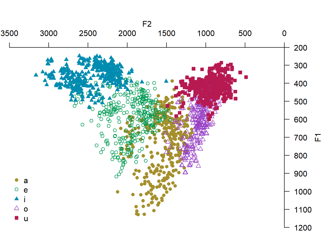

with(indo, plotVowels(f1, f2, var.sty.by = vowel, var.col.by = gender, pretty = TRUE, legend.kwd="bottomleft"))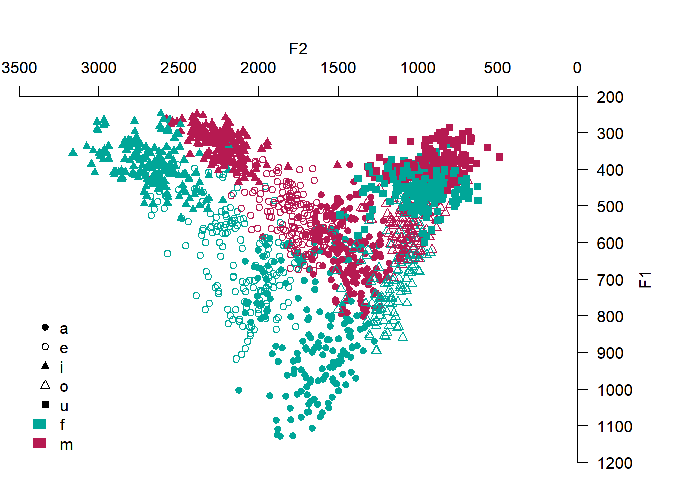

2.9.5 Token means

with(indo, plotVowels(f1, f2, vowel, group = gender, plot.tokens = FALSE, plot.means = TRUE, 
    var.col.by = gender, var.sty.by = vowel, pretty = TRUE, xlim = c(2900, 600), 
    ylim = c(1000, 250), legend.kwd="bottomleft"))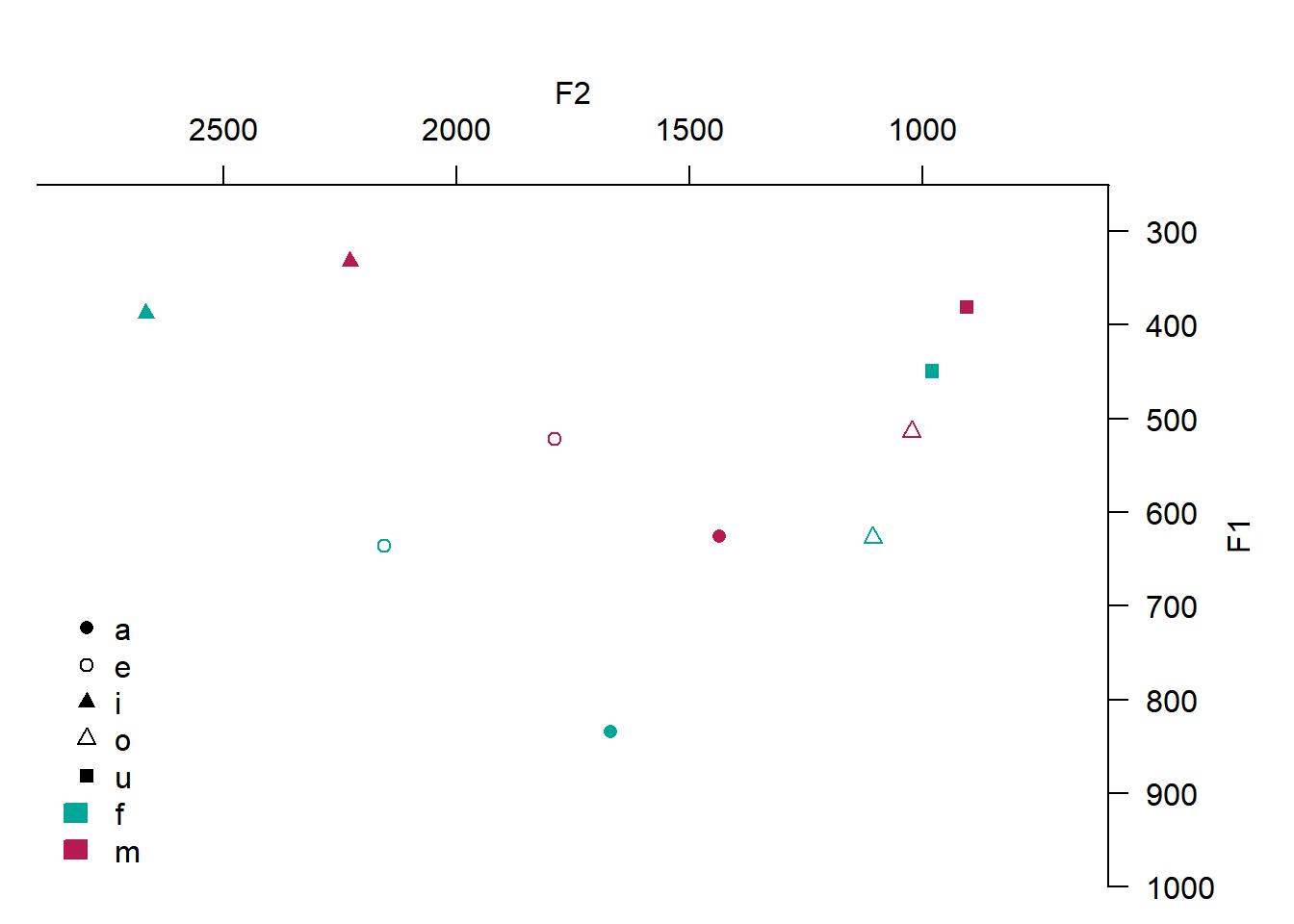

2.9.6 Ellipses and areas

#Ellipses
with(indo, plotVowels(f1, f2, vowel, group = gender, pch.tokens = vowel, cex.tokens = 1.2, 
    alpha.tokens = 0.3, plot.means = TRUE, pch.means = vowel, cex.means = 2, var.col.by = vowel, 
    var.sty.by = gender, hull.fill = TRUE, hull.line = TRUE, fill.opacity = 0.1, 
    pretty = TRUE, legend.kwd = "bottomright"))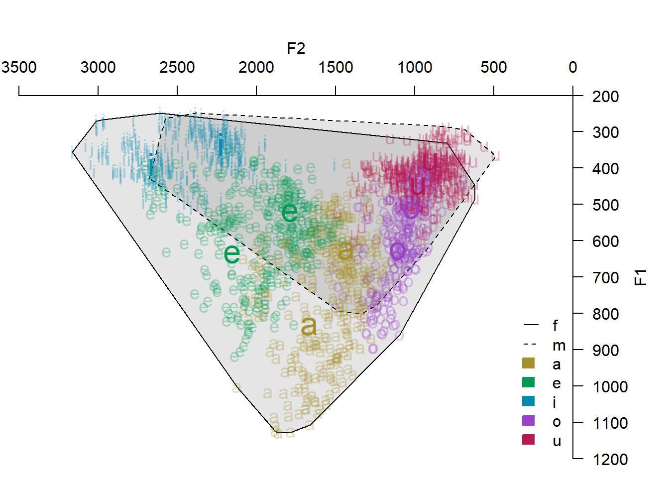

#areas
with(indo, plotVowels(f1, f2, vowel, group = subj, plot.tokens = FALSE, plot.means = TRUE, 
    pch.means = vowel, cex.means = 2, var.col.by = vowel, var.sty.by = subj, ellipse.line = TRUE, 
    ellipse.fill = TRUE, fill.opacity = 0.1, pretty = TRUE, legend.kwd = "bottomright"))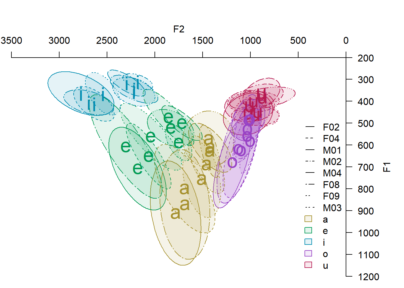

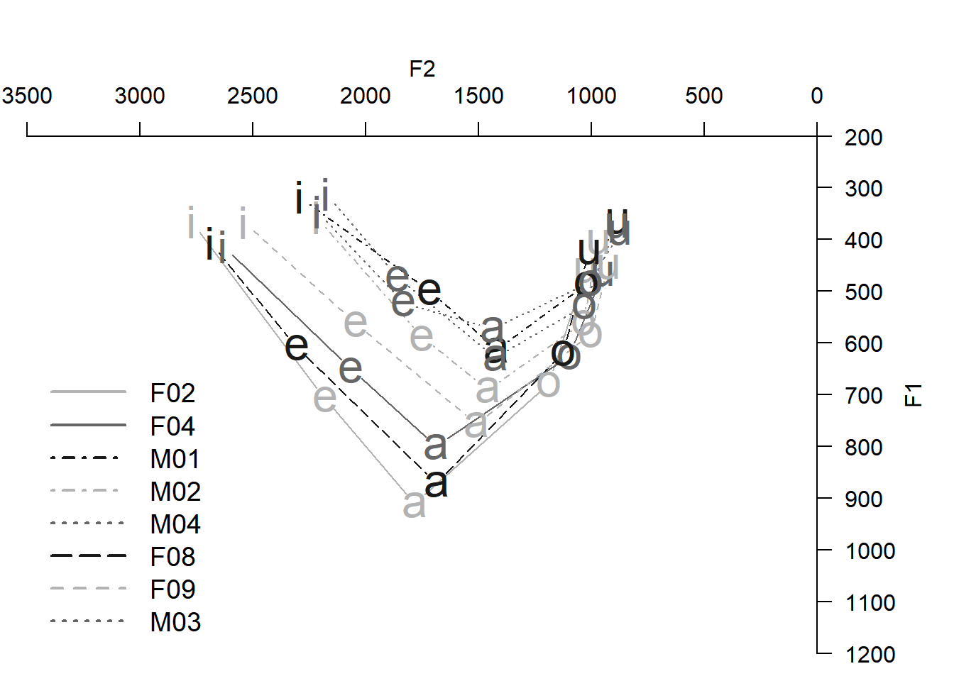
2.9.7 Linking vowels

with(indo, plotVowels(f1, f2, vowel, group = subj, var.col.by = subj, var.sty.by = subj, 
    plot.tokens = FALSE, plot.means = TRUE, pch.means = vowel, cex.means = 2, pretty = TRUE, 
    poly.line = TRUE, poly.order = c("i", "e", "a", "o", "u"), legend.kwd = "bottomleft", 
    legend.args = list(seg.len = 3, cex = 1.2, lwd = 2), col = c("gray70", "gray40", 
        "gray10"), lty = c("solid", "solid", "dotdash", "dotdash", "dotted", "longdash", 
        "dashed", "dotted")))