4.6 Generalised Additive Mixed-effects Models (GAMMs)

Generalised Additive Mixed-effects Models (GAMMs) are currently used for dynamic data. By dynamic data we mean, where the “time” component is accounted for. These can be vowel formants or f0 obtained at 11 intervals; dynamic tongue contours obtained at multiple time points, etc.

We first use GAMMs (with random effects) to demonstrate its usage

4.6.1 Loading dataframe

dynamicDF <- read_csv("data/dynamicData.csv")
dynamicDF %>% 
  head(10)

## # A tibble: 10 × 19
##    Speaker Sex   Word  repetition context vowel Label Duration F2_01 F2_02 F2_03
##    <chr>   <chr> <chr> <chr>      <chr>   <chr> <chr>    <dbl> <dbl> <dbl> <dbl>
##  1 SP01    Male  2aat… rep01      Plain   a:    V2        176. 1500. 1526. 1498.
##  2 SP01    Male  2aat… rep02      Plain   a:    V2        143. 1518. 1520. 1512.
##  3 SP01    Male  2aat… rep03      Plain   a:    V2        108. 1539. 1553. 1556.
##  4 SP01    Male  2aaT… rep01      Pharyn… a:    V2        145. 1046. 1107. 1127.
##  5 SP01    Male  2aaT… rep02      Pharyn… a:    V2        141. 1229. 1242. 1261.
##  6 SP01    Male  2aaT… rep03      Pharyn… a:    V2        108. 1156. 1165. 1171.
##  7 SP01    Male  2iit… rep01      Plain   i:    V2        184. 2269. 2244. 2281.
##  8 SP01    Male  2iit… rep02      Plain   i:    V2        192. 2218. 2197. 2219.
##  9 SP01    Male  2iit… rep03      Plain   i:    V2        172. 2140. 2152. 2182.
## 10 SP01    Male  2iiT… rep01      Pharyn… i:    V2        212. 1337. 1442. 1592.
## # ℹ 8 more variables: F2_04 <dbl>, F2_05 <dbl>, F2_06 <dbl>, F2_07 <dbl>,
## #   F2_08 <dbl>, F2_09 <dbl>, F2_10 <dbl>, F2_11 <dbl>

The dataframe was extracted from a Praat script and comes in a wide format. For it to work properly with GAMMs, we convert it to a long format

4.6.2 Manipulation

4.6.2.1 Wide to Long format

dynamicDF <- dynamicDF %>% 
  pivot_longer(-c(1:8), 
               names_sep = "_",               
               names_to = c("Correlate", "Interval"),
               values_to = "Vals",
               names_repair = "minimal") %>% 
  pivot_wider(names_from = "Correlate", 
              values_from = "Vals") %>% 
  unnest() 
dynamicDF %>% 
  head(10)

## # A tibble: 10 × 10
##    Speaker Sex   Word   repetition context vowel Label Duration Interval    F2
##    <chr>   <chr> <chr>  <chr>      <chr>   <chr> <chr>    <dbl> <chr>    <dbl>
##  1 SP01    Male  2aataa rep01      Plain   a:    V2        176. 01       1500.
##  2 SP01    Male  2aataa rep01      Plain   a:    V2        176. 02       1526.
##  3 SP01    Male  2aataa rep01      Plain   a:    V2        176. 03       1498.
##  4 SP01    Male  2aataa rep01      Plain   a:    V2        176. 04       1462.
##  5 SP01    Male  2aataa rep01      Plain   a:    V2        176. 05       1433.
##  6 SP01    Male  2aataa rep01      Plain   a:    V2        176. 06       1421.
##  7 SP01    Male  2aataa rep01      Plain   a:    V2        176. 07       1419.
##  8 SP01    Male  2aataa rep01      Plain   a:    V2        176. 08       1411.
##  9 SP01    Male  2aataa rep01      Plain   a:    V2        176. 09       1401.
## 10 SP01    Male  2aataa rep01      Plain   a:    V2        176. 10       1428.

4.6.2.2 Transforming and arranging dataframe

dynamicDF <- dynamicDF %>% 
  mutate(Speaker = as.factor(Speaker),
         Sex = as.factor(Sex),
         Word = as.factor(Word),
         repetition = as.factor(repetition),
         context = as.factor(context),
         vowel = as.factor(vowel),
         Interval = as.numeric(Interval)) %>% 
  arrange(Speaker, Word, context, vowel)
dynamicDF %>% 
  head(10)

## # A tibble: 10 × 10
##    Speaker Sex   Word   repetition context vowel Label Duration Interval    F2
##    <fct>   <fct> <fct>  <fct>      <fct>   <fct> <chr>    <dbl>    <dbl> <dbl>
##  1 SP01    Male  2aataa rep01      Plain   a:    V2        176.        1 1500.
##  2 SP01    Male  2aataa rep01      Plain   a:    V2        176.        2 1526.
##  3 SP01    Male  2aataa rep01      Plain   a:    V2        176.        3 1498.
##  4 SP01    Male  2aataa rep01      Plain   a:    V2        176.        4 1462.
##  5 SP01    Male  2aataa rep01      Plain   a:    V2        176.        5 1433.
##  6 SP01    Male  2aataa rep01      Plain   a:    V2        176.        6 1421.
##  7 SP01    Male  2aataa rep01      Plain   a:    V2        176.        7 1419.
##  8 SP01    Male  2aataa rep01      Plain   a:    V2        176.        8 1411.
##  9 SP01    Male  2aataa rep01      Plain   a:    V2        176.        9 1401.
## 10 SP01    Male  2aataa rep01      Plain   a:    V2        176.       10 1428.

4.6.2.3 Ordering predictors

It is important to use an ordered predictor in GAMs. By default, GAMs provides computations similar to an ANOVA (with sum coding). Here, we use a treatment coding to allow for an increase in power. Also, we create an interaction factor; the results are to be modelled as a function of the interaction between the context and the vowel

dynamicDF$ContVowInt <- interaction(dynamicDF$context, dynamicDF$vowel)

dynamicDF$ContVowInt.ord <-  as.ordered(dynamicDF$ContVowInt)  
contrasts(dynamicDF$ContVowInt.ord) <- "contr.treatment"

dynamicDF$Sex.ord <- as.ordered(dynamicDF$Sex)
contrasts(dynamicDF$Sex.ord) <- "contr.treatment"

4.6.2.4 Start value for autocorrelation

Given that time series are heavily correlated, we need to account for this autocorrelation in any analyses. We add a variable “start” to indicate when the Interval == 1

dynamicDF$start <-dynamicDF$Interval == 1

4.6.3 Model specifications

4.6.3.1 No AR1 model

4.6.3.1.1 Model estimation

system.time(mdl.gamm.F2.noAR <- bam(F2 ~ ContVowInt.ord * Sex.ord +
                                      ### 1d smooths
                                      s(Interval, bs = "cr", k = 11) +
                                      ### 1d smooths * factor
                                      s(Interval, bs = "cr", k = 11, by = ContVowInt.ord) +
                                      s(Interval, bs = "cr", k = 11, by = Sex.ord) +
                                      ### random smooths by speaker
                                                                                s(Interval, Speaker, bs = "fs", k = 11, m = 1, xt=list(bs = "tp")) +            s(Interval, Speaker, bs = "fs", k = 11, m = 1, xt=list(bs = "tp"), by = ContVowInt.ord) +
                                     ### random smooths by word
s(Interval, Word, bs = "fs", k = 11, m = 1, xt=list(bs = "tp")) +             s(Interval, Word, bs = "fs", k = 11, m = 1, xt=list(bs = "tp"), by = Sex.ord),
                                      data = dynamicDF, discrete = TRUE, nthreads = 2))

##    user  system elapsed 
##    2.11    0.22    1.99

4.6.3.1.1.1 ACF No AR1

acf_resid(mdl.gamm.F2.noAR, main = "Average ACF No.AR F2",cex.lab=1.5,cex.axis=1.5)

4.6.3.1.1.2 Gam check

gam.check(mdl.gamm.F2.noAR)

## 
## Method: fREML   Optimizer: perf chol
## $grad
##  [1] -2.509104e-14 -2.716716e-13  6.195044e-14 -1.727507e-13  2.042810e-14
##  [6]  1.665335e-14  6.439294e-15 -1.967253e-06  1.110223e-15 -3.167531e-06
## [11]  4.440892e-16 -6.572520e-14 -2.886580e-15 -3.165860e-06  1.998401e-15
## [16] -5.551115e-14  4.662937e-15 -3.663736e-14  4.218847e-15 -2.561403e-06
## [21]  1.332268e-15 -3.476698e-06  1.110223e-14  3.555556e-11
## 
## $hess
##            [,1]          [,2]          [,3]          [,4]          [,5]
##    1.003880e+00 -9.361499e-02  9.867539e-03 -1.773653e-01  1.813204e-02
##   -9.361499e-02  1.638108e-01  2.307914e-02 -6.348586e-02 -4.914258e-02
##    9.867539e-03  2.307914e-02  1.193923e+00  1.370215e-02  2.170922e-02
##   -1.773653e-01 -6.348586e-02  1.370215e-02  3.473970e-01 -4.569094e-03
##    1.813204e-02 -4.914258e-02  2.170922e-02 -4.569094e-03  1.105819e+00
##    1.869996e-02 -4.161598e-02  1.925866e-02 -1.293336e-03 -5.549452e-02
##   -2.506757e-01 -9.568044e-03  2.012076e-03  3.342137e-02 -3.534940e-02
##    1.835864e-06 -2.041012e-08 -6.795749e-08 -4.024643e-07  2.384429e-07
##   -4.200960e-27 -1.253884e-28 -3.465254e-28  8.942480e-28  3.098441e-28
##    4.388010e-08  2.222766e-07  2.794168e-08 -5.336235e-08 -8.684646e-08
##    4.200961e-28 -1.267902e-28 -1.105661e-28  3.623517e-28 -3.389264e-29
##   -2.094426e-02 -3.873479e-03  6.382315e-02  4.224116e-03 -8.042748e-03
##   -2.430787e-28  3.097148e-29 -3.098978e-27 -3.389654e-29  2.874610e-29
##    2.724867e-08 -2.343219e-08  2.858970e-09  1.451438e-07  2.394565e-08
##   -3.241300e-27 -4.534158e-29  3.265520e-28  8.036604e-27  1.046087e-28
##   -2.111491e-02  5.202241e-03 -8.566203e-04  1.013440e-03  7.873933e-02
##   -5.321192e-28  2.645573e-29  5.970949e-29 -9.247070e-29  4.219779e-28
##   -2.067744e-02  3.927096e-03 -9.736665e-04  7.681664e-04  3.362567e-03
##   -9.413504e-29  7.010344e-30  2.400520e-29 -3.469041e-29 -8.631820e-30
##    1.666934e-06  1.956228e-06 -3.382783e-07  1.774858e-06  7.445482e-07
##    4.748185e-27  5.546130e-28 -2.857531e-27  4.020928e-27  2.489835e-28
##    3.217140e-08  1.535342e-07 -5.404928e-08  2.378842e-07 -1.894141e-07
##   -4.727416e-29 -2.206049e-28 -3.817662e-28  2.079086e-27  4.536311e-29
## d -1.050806e+00 -3.614705e-01 -1.228224e+00 -5.976267e-01 -1.231656e+00
##            [,6]          [,7]          [,8]          [,9]         [,10]
##    1.869996e-02 -2.506757e-01  1.835864e-06 -4.248753e-27  4.388010e-08
##   -4.161598e-02 -9.568044e-03 -2.041012e-08 -1.265055e-28  2.222766e-07
##    1.925866e-02  2.012076e-03 -6.795749e-08 -5.301576e-28  2.794168e-08
##   -1.293336e-03  3.342137e-02 -4.024643e-07  8.667962e-28 -5.336235e-08
##   -5.549452e-02 -3.534940e-02  2.384429e-07  2.196814e-28 -8.684646e-08
##    1.608696e+00 -3.333043e-02  1.906263e-07  3.116542e-28 -7.452219e-08
##   -3.333043e-02  7.405700e-01  2.946194e-06 -4.695326e-27  7.542137e-08
##    1.906263e-07  2.946194e-06  1.967272e-06 -5.321578e-32  8.682268e-13
##    3.110792e-28 -4.748096e-27 -5.356664e-32 -1.110223e-15 -2.628689e-33
##   -7.452219e-08  7.542137e-08  8.682268e-13 -1.834629e-33  3.167528e-06
##   -2.688042e-29 -1.078047e-27 -2.888068e-33 -2.230640e-29  8.255722e-33
##   -7.722929e-03 -1.301421e-01 -1.302448e-06 -2.929285e-27  9.333260e-08
##   -1.395514e-29 -4.117124e-28 -2.308468e-33 -1.958972e-29  3.424957e-34
##    2.308512e-08  2.387087e-07 -2.472654e-14 -7.249245e-34 -1.729391e-12
##    7.464619e-29 -1.699484e-27 -2.907516e-32 -8.392858e-30 -1.131031e-32
##    3.106205e-03  4.813115e-02  7.265923e-07 -1.507880e-27  2.598147e-07
##   -1.446736e-29 -6.379518e-28 -6.756731e-33 -1.797712e-29 -8.025106e-34
##    3.593009e-02  1.859382e-02  2.987398e-07 -3.858902e-28  5.042282e-07
##    2.708966e-28  1.235142e-29 -4.625228e-34 -1.022599e-29  4.831796e-35
##    4.889666e-07 -2.577409e-07  1.250788e-12 -4.198249e-33  2.557888e-12
##   -2.753673e-28 -1.934986e-27  1.221272e-32 -3.775948e-29  6.548766e-33
##   -1.251857e-07  8.775859e-08  2.813470e-13 -1.281770e-33 -1.753342e-12
##   -1.308204e-28  3.572530e-28  2.044900e-33 -1.179930e-28  2.223466e-32
## d -1.564357e+00 -1.031287e+00 -8.032182e-06 -1.970043e-24 -2.306632e-06
##           [,11]         [,12]         [,13]         [,14]         [,15]
##    4.293231e-28 -2.094426e-02 -2.454962e-28  2.724867e-08 -3.210420e-27
##   -1.500579e-28 -3.873479e-03  2.003625e-31 -2.343219e-08 -2.197492e-29
##   -1.130741e-28  6.382315e-02 -2.051043e-27  2.858970e-09  3.251609e-28
##    3.675007e-28  4.224116e-03 -5.203579e-29  1.451438e-07  8.063222e-27
##   -3.321400e-29 -8.042748e-03  8.525615e-31  2.394565e-08  1.172171e-28
##   -2.519244e-29 -7.722929e-03 -3.319423e-30  2.308512e-08  8.141685e-29
##   -1.080657e-27 -1.301421e-01 -3.619740e-28  2.387087e-07 -1.688159e-27
##   -2.840469e-33 -1.302448e-06 -5.646954e-33 -2.472654e-14 -3.042376e-32
##   -2.230640e-29 -3.079636e-27 -1.958972e-29 -7.021621e-34 -8.392858e-30
##    8.144441e-33  9.333260e-08  2.578803e-34 -1.729391e-12 -1.110518e-32
##   -4.440892e-16  1.155631e-28 -1.218217e-34  1.193419e-33 -1.459821e-34
##    1.153928e-28  5.713580e+00 -1.474677e-26 -1.406852e-07  9.407985e-28
##   -1.218217e-34 -1.429791e-26  2.886580e-15  1.497593e-34 -1.185236e-34
##    1.195054e-33 -1.406852e-07  1.491763e-35  3.165853e-06 -4.974363e-33
##   -1.459821e-34  9.513352e-28 -1.185236e-34 -4.618614e-33 -1.998401e-15
##    2.380889e-28  7.439112e-02  2.571311e-29  1.100026e-07  6.498501e-28
##   -4.340829e-34  1.690408e-28 -1.719480e-34  5.151124e-34 -4.919951e-34
##    4.495824e-28  3.620299e-02 -3.800957e-30  3.157134e-08  1.876200e-27
##   -5.590015e-35  1.783161e-29 -4.560896e-34 -1.523701e-35 -2.110598e-34
##    5.015382e-33 -2.180195e-07 -3.569024e-34  9.876859e-13  4.319863e-32
##   -2.839017e-29 -2.148683e-27 -2.245794e-29  4.980048e-33 -3.436068e-29
##    3.236505e-33  1.061986e-07 -1.191646e-34 -3.065580e-12 -9.056812e-33
##   -3.984237e-29  1.489678e-27 -1.411590e-29  1.057010e-32 -1.921045e-29
## d -1.926112e-25 -6.080384e+00 -3.757426e-24 -1.694360e-06 -4.341190e-24
##           [,16]         [,17]         [,18]         [,19]         [,20]
##   -2.111491e-02 -5.343174e-28 -2.067744e-02 -1.012711e-28  1.666934e-06
##    5.202241e-03  2.322106e-29  3.927096e-03  7.344965e-30  1.956228e-06
##   -8.566203e-04  5.829701e-29 -9.736665e-04  2.454509e-29 -3.382783e-07
##    1.013440e-03 -9.661887e-29  7.681664e-04 -3.679830e-29  1.774858e-06
##    7.873933e-02  4.050782e-28  3.362567e-03 -7.331899e-30  7.445482e-07
##    3.106205e-03 -1.405435e-29  3.593009e-02  2.782205e-28  4.889666e-07
##    4.813115e-02 -6.370116e-28  1.859382e-02  8.727449e-30 -2.577409e-07
##    7.265923e-07 -7.483849e-33  2.987398e-07 -2.758950e-34  1.250788e-12
##   -1.467307e-27 -1.797712e-29  2.814182e-29 -1.022599e-29 -4.245444e-33
##    2.598147e-07 -6.260476e-34  5.042282e-07  3.771134e-36  2.557888e-12
##    2.375394e-28 -4.340829e-34  4.383456e-28 -5.590015e-35  4.756450e-33
##    7.439112e-02  1.680131e-28  3.620299e-02  1.889467e-29 -2.180195e-07
##    1.772335e-29 -1.719480e-34  6.683440e-29 -4.560896e-34 -6.805432e-34
##    1.100026e-07  4.887320e-34  3.157134e-08 -4.571799e-36  9.876859e-13
##    7.723775e-28 -4.919951e-34  1.926726e-27 -2.110598e-34  4.417539e-32
##    9.728958e-01 -2.323578e-27 -1.056477e-01 -1.197128e-29 -1.796839e-07
##   -2.397561e-27 -4.662937e-15  8.769651e-29 -1.023935e-34  1.416348e-33
##   -1.056477e-01  1.110312e-28  1.681829e+00 -1.348547e-28 -1.688652e-07
##   -1.368128e-29 -1.023935e-34 -1.302854e-28 -4.218847e-15  5.042038e-34
##   -1.796839e-07  1.571989e-33 -1.688652e-07  3.840613e-34  2.561441e-06
##    4.670724e-28 -2.230883e-28 -2.006339e-28 -3.973874e-29  4.773614e-32
##    3.614614e-07 -6.346832e-34  6.800200e-07 -1.380818e-34  2.983844e-12
##    4.619700e-28 -3.378369e-29 -1.474383e-27 -3.224206e-29  1.336938e-32
## d -1.725493e+00 -8.539325e-25 -1.827487e+00 -1.319997e-25 -1.206302e-05
##           [,21]         [,22]         [,23]         [,24]
##    4.580460e-27  3.217140e-08 -1.771389e-29 -1.050806e+00
##    5.070990e-28  1.535342e-07 -2.554026e-28 -3.614705e-01
##   -2.310227e-27 -5.404928e-08 -3.851550e-28 -1.228224e+00
##    4.001775e-27  2.378842e-07  2.083697e-27 -5.976267e-01
##    3.600963e-28 -1.894141e-07  5.143670e-29 -1.231656e+00
##   -2.052313e-28 -1.251857e-07 -1.449697e-28 -1.564357e+00
##   -1.999159e-27  8.775859e-08  3.620552e-28 -1.031287e+00
##    1.374754e-32  2.813470e-13  1.846941e-33 -8.032182e-06
##   -3.775948e-29 -1.628886e-33 -1.179930e-28 -1.970043e-24
##    6.618090e-33 -1.753342e-12  2.146491e-32 -2.306632e-06
##   -2.839017e-29  3.244701e-33 -3.984237e-29 -1.926112e-25
##   -2.076595e-27  1.061986e-07  1.508691e-27 -6.080384e+00
##   -2.245794e-29  3.629973e-35 -1.411590e-29 -3.757426e-24
##    4.785969e-33 -3.065580e-12  1.071426e-32 -1.694360e-06
##   -3.436068e-29 -9.036936e-33 -1.921045e-29 -4.341190e-24
##    4.795680e-28  3.614614e-07  4.472073e-28 -1.725493e+00
##   -2.230883e-28 -1.188917e-33 -3.378369e-29 -8.539325e-25
##   -5.584062e-29  6.800200e-07 -1.425695e-27 -1.827487e+00
##   -3.973874e-29 -1.633791e-34 -3.224206e-29 -1.319997e-25
##    4.980603e-32  2.983844e-12  1.366492e-32 -1.206302e-05
##   -1.776357e-15  6.788526e-33 -4.858773e-28 -3.985559e-24
##    6.441804e-33  3.476696e-06  1.313330e-32 -2.851468e-06
##   -4.858773e-28  1.323177e-32 -1.110223e-14 -9.860271e-25
## d -3.985559e-24 -2.851468e-06 -9.860271e-25  1.885000e+02
## 
## Model rank =  346 / 346 
## 
## Basis dimension (k) checking results. Low p-value (k-index<1) may
## indicate that k is too low, especially if edf is close to k'.
## 
##                                                           k'      edf k-index
## s(Interval)                                         1.00e+01 3.10e+00    1.29
## s(Interval):ContVowInt.ordPlain.a:                  1.00e+01 1.72e+00    1.29
## s(Interval):ContVowInt.ordPharyngealised.i:         1.00e+01 3.46e+00    1.29
## s(Interval):ContVowInt.ordPlain.i:                  1.00e+01 2.20e+00    1.29
## s(Interval):ContVowInt.ordPharyngealised.u:         1.00e+01 3.46e+00    1.29
## s(Interval):ContVowInt.ordPlain.u:                  1.00e+01 4.13e+00    1.29
## s(Interval):Sex.ordMale                             1.00e+01 3.06e+00    1.29
## s(Interval,Speaker)                                 2.20e+01 2.00e-05    1.29
## s(Interval,Speaker):ContVowInt.ordPlain.a:          2.20e+01 1.10e-05    1.29
## s(Interval,Speaker):ContVowInt.ordPharyngealised.i: 2.20e+01 1.22e+01    1.29
## s(Interval,Speaker):ContVowInt.ordPlain.i:          2.20e+01 9.72e-06    1.29
## s(Interval,Speaker):ContVowInt.ordPharyngealised.u: 2.20e+01 3.45e+00    1.29
## s(Interval,Speaker):ContVowInt.ordPlain.u:          2.20e+01 3.65e+00    1.29
## s(Interval,Word)                                    6.60e+01 2.92e-05    1.29
## s(Interval,Word):Sex.ordMale                        6.60e+01 1.27e-05    1.29
##                                                     p-value
## s(Interval)                                               1
## s(Interval):ContVowInt.ordPlain.a:                        1
## s(Interval):ContVowInt.ordPharyngealised.i:               1
## s(Interval):ContVowInt.ordPlain.i:                        1
## s(Interval):ContVowInt.ordPharyngealised.u:               1
## s(Interval):ContVowInt.ordPlain.u:                        1
## s(Interval):Sex.ordMale                                   1
## s(Interval,Speaker)                                       1
## s(Interval,Speaker):ContVowInt.ordPlain.a:                1
## s(Interval,Speaker):ContVowInt.ordPharyngealised.i:       1
## s(Interval,Speaker):ContVowInt.ordPlain.i:                1
## s(Interval,Speaker):ContVowInt.ordPharyngealised.u:       1
## s(Interval,Speaker):ContVowInt.ordPlain.u:                1
## s(Interval,Word)                                          1
## s(Interval,Word):Sex.ordMale                              1

4.6.3.1.1.3 Estimating Rho

rho_est <- start_value_rho(mdl.gamm.F2.noAR)
rho_est

## [1] 0.715958

4.6.3.2 AR1 model

4.6.3.2.0.1 Model estimation

system.time(mdl.gamm.F2.AR <- bam(F2 ~ ContVowInt.ord * Sex.ord +
                                      ### 1d smooths
                                      s(Interval, bs = "cr", k = 11) +
                                      ### 1d smooths * factor
                                      s(Interval, bs = "cr", k = 11, by = ContVowInt.ord) +
                                      s(Interval, bs = "cr", k = 11, by = Sex.ord) +
                                      ### random smooths by speaker
                                                                                s(Interval, Speaker, bs = "fs", k = 11, m = 1, xt=list(bs = "tp")) +            s(Interval, Speaker, bs = "fs", k = 11, m = 1, xt=list(bs = "tp"), by = ContVowInt.ord) +
                                     ### random smooths by word
s(Interval, Word, bs = "fs", k = 11, m = 1, xt=list(bs = "tp")) +             s(Interval, Word, bs = "fs", k = 11, m = 1, xt=list(bs = "tp"), by = Sex.ord), data = dynamicDF, discrete = TRUE, nthreads = 2, AR.start = dynamicDF$start, rho = rho_est))

##    user  system elapsed 
##    1.11    0.11    1.02

4.6.3.2.0.2 ACF AR1

acf_resid(mdl.gamm.F2.AR, main = "Average ACF AR F2",cex.lab=1.5,cex.axis=1.5)

4.6.3.2.0.3 Summary

summary(mdl.gamm.F2.AR)

Family: gaussian Link function: identity

Formula: F2 ~ ContVowInt.ord * Sex.ord + s(Interval, bs = “cr”, k = 11) + s(Interval, bs = “cr”, k = 11, by = ContVowInt.ord) + s(Interval, bs = “cr”, k = 11, by = Sex.ord) + s(Interval, Speaker, bs = “fs”, k = 11, m = 1, xt = list(bs = “tp”)) + s(Interval, Speaker, bs = “fs”, k = 11, m = 1, xt = list(bs = “tp”), by = ContVowInt.ord) + s(Interval, Word, bs = “fs”, k = 11, m = 1, xt = list(bs = “tp”)) + s(Interval, Word, bs = “fs”, k = 11, m = 1, xt = list(bs = “tp”), by = Sex.ord)

Parametric coefficients: Estimate Std. Error t value (Intercept) 1318.57 17.74 74.322 ContVowInt.ordPlain.a: 259.70 27.35 9.496 ContVowInt.ordPharyngealised.i: 999.04 27.59 36.204 ContVowInt.ordPlain.i: 1244.99 27.44 45.364 ContVowInt.ordPharyngealised.u: -399.49 27.45 -14.553 ContVowInt.ordPlain.u: -266.02 27.50 -9.673 Sex.ordMale -147.62 24.95 -5.916 ContVowInt.ordPlain.a::Sex.ordMale 70.77 38.41 1.842 ContVowInt.ordPharyngealised.i::Sex.ordMale -226.37 38.93 -5.815 ContVowInt.ordPlain.i::Sex.ordMale -135.40 38.59 -3.509 ContVowInt.ordPharyngealised.u::Sex.ordMale 78.25 38.52 2.031 ContVowInt.ordPlain.u::Sex.ordMale 42.06 38.66 1.088 Pr(>|t|)
(Intercept) < 2e-16 ContVowInt.ordPlain.a: < 2e-16 ContVowInt.ordPharyngealised.i: < 2e-16 ContVowInt.ordPlain.i: < 2e-16 ContVowInt.ordPharyngealised.u: < 2e-16 ContVowInt.ordPlain.u: < 2e-16 Sex.ordMale 8.34e-09 ContVowInt.ordPlain.a::Sex.ordMale 0.066332 .
ContVowInt.ordPharyngealised.i::Sex.ordMale 1.44e-08 ContVowInt.ordPlain.i::Sex.ordMale 0.000513 ** ContVowInt.ordPharyngealised.u::Sex.ordMale 0.043038
ContVowInt.ordPlain.u::Sex.ordMale 0.277405
— Signif. codes: 0 ‘’ 0.001 ’’ 0.01 ’’ 0.05 ‘.’ 0.1 ’ ’ 1

Approximate significance of smooth terms: edf Ref.df F s(Interval) 4.524e+00 5.638 12.737 s(Interval):ContVowInt.ordPlain.a: 2.434e+00 3.185 2.310 s(Interval):ContVowInt.ordPharyngealised.i: 3.507e+00 3.582 11.934 s(Interval):ContVowInt.ordPlain.i: 2.884e+00 3.567 10.334 s(Interval):ContVowInt.ordPharyngealised.u: 5.193e+00 6.419 10.664 s(Interval):ContVowInt.ordPlain.u: 5.735e+00 6.684 19.337 s(Interval):Sex.ordMale 5.009e+00 6.197 14.079 s(Interval,Speaker) 1.242e-05 19.000 0.000 s(Interval,Speaker):ContVowInt.ordPlain.a: 7.557e-06 21.000 0.000 s(Interval,Speaker):ContVowInt.ordPharyngealised.i: 1.547e+01 19.000 13.759 s(Interval,Speaker):ContVowInt.ordPlain.i: 4.679e+00 19.000 0.332 s(Interval,Speaker):ContVowInt.ordPharyngealised.u: 2.548e+00 19.000 0.164 s(Interval,Speaker):ContVowInt.ordPlain.u: 5.691e+00 19.000 0.573 s(Interval,Word) 1.378e-05 59.000 0.000 s(Interval,Word):Sex.ordMale 1.132e-05 65.000 0.000 p-value
s(Interval) < 2e-16 s(Interval):ContVowInt.ordPlain.a: 0.0661 .
s(Interval):ContVowInt.ordPharyngealised.i: < 2e-16 s(Interval):ContVowInt.ordPlain.i: 7.13e-07 s(Interval):ContVowInt.ordPharyngealised.u: < 2e-16 s(Interval):ContVowInt.ordPlain.u: < 2e-16 s(Interval):Sex.ordMale < 2e-16 s(Interval,Speaker) 0.2584
s(Interval,Speaker):ContVowInt.ordPlain.a: 0.8747
s(Interval,Speaker):ContVowInt.ordPharyngealised.i: < 2e-16 * s(Interval,Speaker):ContVowInt.ordPlain.i: 0.0910 .
s(Interval,Speaker):ContVowInt.ordPharyngealised.u: 0.1405
s(Interval,Speaker):ContVowInt.ordPlain.u: 0.0073 s(Interval,Word) 0.7046
s(Interval,Word):Sex.ordMale 0.5256
— Signif. codes: 0 ‘’ 0.001 ’’ 0.01 ’’ 0.05 ‘.’ 0.1 ’ ’ 1

R-sq.(adj) = 0.993 Deviance explained = 99.4% fREML = 1856.4 Scale est. = 1469.1 n = 396

4.6.3.2.0.4 Model’s fit

print(tab_model(mdl.gamm.F2.AR, file = paste0("outputs/mdl.gamm.F2.AR.html")))
htmltools::includeHTML("outputs/mdl.gamm.F2.AR.html")

	F 2
Predictors	Estimates	CI	p
(Intercept)	1318.57	1283.66 – 1353.47	<0.001
ContVowInt ordPlain a	259.70	205.90 – 313.50	<0.001
ContVowInt ordPharyngealised i	999.04	944.76 – 1053.33	<0.001
ContVowInt ordPlain i	1244.99	1191.00 – 1298.98	<0.001
ContVowInt ordPharyngealised u	-399.49	-453.50 – -345.49	<0.001
ContVowInt ordPlain u	-266.02	-320.12 – -211.92	<0.001
Sex ord [Male]	-147.62	-196.71 – -98.53	<0.001
Sex ord [Male]	70.77	-4.80 – 146.33	0.066
Sex ord [Male]	-226.37	-302.94 – -149.79	<0.001
Sex ord [Male]	-135.40	-211.32 – -59.49	0.001
Sex ord [Male]	78.25	2.47 – 154.04	0.043
Sex ord [Male]	42.06	-33.99 – 118.11	0.277
s(Interval)			<0.001
s(Interval) × ContVowInt ordPlain a			0.066
s(Interval) × ContVowInt ordPharyngealised i			<0.001
s(Interval) × ContVowInt ordPlain i			<0.001
s(Interval) × ContVowInt ordPharyngealised u			<0.001
s(Interval) × ContVowInt ordPlain u			<0.001
s(Interval) × Sex ord [Male]			<0.001
s(Interval,Speaker)			0.258
s(Interval,Speaker) × ContVowInt ordPlain a			0.875
s(Interval,Speaker) × ContVowInt ordPharyngealised i			<0.001
s(Interval,Speaker) × ContVowInt ordPlain i			0.091
s(Interval,Speaker) × ContVowInt ordPharyngealised u			0.141
s(Interval,Speaker) × ContVowInt ordPlain u			0.007
s(Interval,Word)			0.705
s(Interval,Word) × Sex ord [Male]			0.526
Observations	396
R2	0.993

4.6.4 Significance testing second Autoregressive GAM

To test for significance of context, we run a model with a ML as method and evaluate significance through a maximum likelihood estimate.

4.6.4.1 Models

We run two models

1. A full model with all predictors (mdl.gamm.F2.AR.ML)
2. A reduced model without any terms associated with the predictor “context” (mdl.gamm.F2.AR.Min.ContVowInt.ord.ML)
3. An intercept only model (=Null) without any terms associated with the predictor “vowel” (mdl.gamm.F2.AR.Min.ContVowInt.ord.Sex.ord.ML)

4.6.4.1.1 Full Model

system.time(mdl.gamm.F2.AR.ML <- bam(F2 ~ ContVowInt.ord * Sex.ord +
                                      ### 1d smooths
                                      s(Interval, bs = "cr", k = 11) +
                                      ### 1d smooths * factor
                                      s(Interval, bs = "cr", k = 11, by = ContVowInt.ord) +
                                      s(Interval, bs = "cr", k = 11, by = Sex.ord) +
                                      ### random smooths by speaker
                                                                                s(Interval, Speaker, bs = "fs", k = 11, m = 1, xt=list(bs = "tp")) +            s(Interval, Speaker, bs = "fs", k = 11, m = 1, xt=list(bs = "tp"), by = ContVowInt.ord) +
                                     ### random smooths by word
s(Interval, Word, bs = "fs", k = 11, m = 1, xt=list(bs = "tp")) +             s(Interval, Word, bs = "fs", k = 11, m = 1, xt=list(bs = "tp"), by = Sex.ord), data = dynamicDF, discrete = TRUE, nthreads = 2, AR.start = dynamicDF$start, rho = rho_est, method="ML"))

##    user  system elapsed 
##   23.62    0.70   22.47

4.6.4.1.2 Model 2 (without ConVowelInt.ord)

system.time(mdl.gamm.F2.AR.Min.ContVowInt.ord.ML <- bam(F2 ~ Sex.ord +
                                      ### 1d smooths
                                      s(Interval, bs = "cr", k = 11) +
                                      ### 1d smooths * factor
                                      s(Interval, bs = "cr", k = 11, by = Sex.ord) +
                                      ### random smooths by speaker
                                                                                s(Interval, Speaker, bs = "fs", k = 11, m = 1, xt=list(bs = "tp")) +   
                                     ### random smooths by word
s(Interval, Word, bs = "fs", k = 11, m = 1, xt=list(bs = "tp")) +             s(Interval, Word, bs = "fs", k = 11, m = 1, xt=list(bs = "tp"), by = Sex.ord), data = dynamicDF, discrete = TRUE, nthreads = 2, AR.start = dynamicDF$start, rho = rho_est, method="ML"))

##    user  system elapsed 
##    4.95    0.42    6.18

4.6.4.1.3 Null Model

system.time(mdl.gamm.F2.AR.Min.ContVowInt.ord.Sex.ord.ML <- bam(F2 ~ 
                                      ### 1d smooths
                                      s(Interval, bs = "cr", k = 11) +
                                      ### 1d smooths * factor
                                      ### random smooths by speaker
                                                                                s(Interval, Speaker, bs = "fs", k = 11, m = 1, xt=list(bs = "tp")) +    
                                     ### random smooths by word
s(Interval, Word, bs = "fs", k = 11, m = 1, xt=list(bs = "tp")), data = dynamicDF, discrete = TRUE, nthreads = 2, AR.start = dynamicDF$start, rho = rho_est, method="ML"))

##    user  system elapsed 
##    1.44    0.44    2.37

4.6.4.2 Testing significance

compareML(mdl.gamm.F2.AR.ML, mdl.gamm.F2.AR.Min.ContVowInt.ord.ML)

## mdl.gamm.F2.AR.ML: F2 ~ ContVowInt.ord * Sex.ord + s(Interval, bs = "cr", k = 11) + 
##     s(Interval, bs = "cr", k = 11, by = ContVowInt.ord) + s(Interval, 
##     bs = "cr", k = 11, by = Sex.ord) + s(Interval, Speaker, bs = "fs", 
##     k = 11, m = 1, xt = list(bs = "tp")) + s(Interval, Speaker, 
##     bs = "fs", k = 11, m = 1, xt = list(bs = "tp"), by = ContVowInt.ord) + 
##     s(Interval, Word, bs = "fs", k = 11, m = 1, xt = list(bs = "tp")) + 
##     s(Interval, Word, bs = "fs", k = 11, m = 1, xt = list(bs = "tp"), 
##         by = Sex.ord)
## 
## mdl.gamm.F2.AR.Min.ContVowInt.ord.ML: F2 ~ Sex.ord + s(Interval, bs = "cr", k = 11) + s(Interval, bs = "cr", 
##     k = 11, by = Sex.ord) + s(Interval, Speaker, bs = "fs", k = 11, 
##     m = 1, xt = list(bs = "tp")) + s(Interval, Word, bs = "fs", 
##     k = 11, m = 1, xt = list(bs = "tp")) + s(Interval, Word, 
##     bs = "fs", k = 11, m = 1, xt = list(bs = "tp"), by = Sex.ord)
## 
## Chi-square test of ML scores
## -----
##                                  Model    Score Edf Difference     Df  p.value
## 1 mdl.gamm.F2.AR.Min.ContVowInt.ord.ML 2082.786  12                           
## 2                    mdl.gamm.F2.AR.ML 1930.850  42    151.936 30.000  < 2e-16
##   Sig.
## 1     
## 2  ***
## 
## AIC difference: -57.04, model mdl.gamm.F2.AR.ML has lower AIC.

compareML(mdl.gamm.F2.AR.ML, mdl.gamm.F2.AR.Min.ContVowInt.ord.Sex.ord.ML)

## mdl.gamm.F2.AR.ML: F2 ~ ContVowInt.ord * Sex.ord + s(Interval, bs = "cr", k = 11) + 
##     s(Interval, bs = "cr", k = 11, by = ContVowInt.ord) + s(Interval, 
##     bs = "cr", k = 11, by = Sex.ord) + s(Interval, Speaker, bs = "fs", 
##     k = 11, m = 1, xt = list(bs = "tp")) + s(Interval, Speaker, 
##     bs = "fs", k = 11, m = 1, xt = list(bs = "tp"), by = ContVowInt.ord) + 
##     s(Interval, Word, bs = "fs", k = 11, m = 1, xt = list(bs = "tp")) + 
##     s(Interval, Word, bs = "fs", k = 11, m = 1, xt = list(bs = "tp"), 
##         by = Sex.ord)
## 
## mdl.gamm.F2.AR.Min.ContVowInt.ord.Sex.ord.ML: F2 ~ s(Interval, bs = "cr", k = 11) + s(Interval, Speaker, bs = "fs", 
##     k = 11, m = 1, xt = list(bs = "tp")) + s(Interval, Word, 
##     bs = "fs", k = 11, m = 1, xt = list(bs = "tp"))
## 
## Chi-square test of ML scores
## -----
##                                          Model    Score Edf Difference     Df
## 1 mdl.gamm.F2.AR.Min.ContVowInt.ord.Sex.ord.ML 2150.456   7                  
## 2                            mdl.gamm.F2.AR.ML 1930.850  42    219.606 35.000
##    p.value Sig.
## 1              
## 2  < 2e-16  ***
## 
## AIC difference: -327.96, model mdl.gamm.F2.AR.ML has lower AIC.

4.6.5 Visualising smooths

4.6.5.1 /i:/

plot_smooth(mdl.gamm.F2.AR, view = "Interval", cond = list(ContVowInt.ord = "Plain.i:"), col = "blue", ylab = "", xlab = "", main = "GAMM smooths in /i:/ ", hide.label = TRUE, cex.axis = 1.3, ylim = c(1700, 2800), rm.ranef = TRUE)

## Summary:
##  * ContVowInt.ord : factor; set to the value(s): Plain.i:. 
##  * Sex.ord : factor; set to the value(s): Female. 
##  * Interval : numeric predictor; with 30 values ranging from 1.000000 to 11.000000. 
##  * Speaker : factor; set to the value(s): SP01. (Might be canceled as random effect, check below.) 
##  * Word : factor; set to the value(s): 2aataa. (Might be canceled as random effect, check below.) 
##  * NOTE : The following random effects columns are canceled: s(Interval,Speaker),s(Interval,Speaker):ContVowInt.ordPlain.a:,s(Interval,Speaker):ContVowInt.ordPharyngealised.i:,s(Interval,Speaker):ContVowInt.ordPlain.i:,s(Interval,Speaker):ContVowInt.ordPharyngealised.u:,s(Interval,Speaker):ContVowInt.ordPlain.u:,s(Interval,Word),s(Interval,Word):Sex.ordMale
## 

## Note: Selection of grouping predictors does not seem to appear in data. Rug of all data is being added.

plot_smooth(mdl.gamm.F2.AR, view = "Interval", cond = list(ContVowInt.ord = "Pharyngealised.i:"), col = "red", ylab = "", xlab = "", hide.label = TRUE, cex.axis = 1.3, ylim = c(1700, 2800), rm.ranef = TRUE, add = TRUE)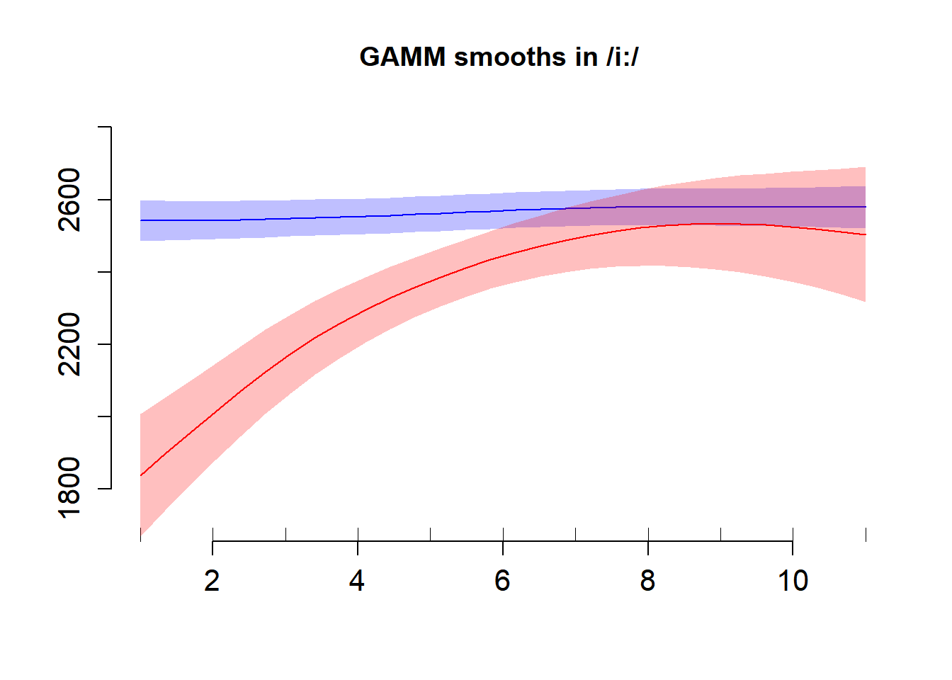

## Summary:
##  * ContVowInt.ord : factor; set to the value(s): Pharyngealised.i:. 
##  * Sex.ord : factor; set to the value(s): Female. 
##  * Interval : numeric predictor; with 30 values ranging from 1.000000 to 11.000000. 
##  * Speaker : factor; set to the value(s): SP01. (Might be canceled as random effect, check below.) 
##  * Word : factor; set to the value(s): 2aataa. (Might be canceled as random effect, check below.) 
##  * NOTE : The following random effects columns are canceled: s(Interval,Speaker),s(Interval,Speaker):ContVowInt.ordPlain.a:,s(Interval,Speaker):ContVowInt.ordPharyngealised.i:,s(Interval,Speaker):ContVowInt.ordPlain.i:,s(Interval,Speaker):ContVowInt.ordPharyngealised.u:,s(Interval,Speaker):ContVowInt.ordPlain.u:,s(Interval,Word),s(Interval,Word):Sex.ordMale
##  
## Note: Selection of grouping predictors does not seem to appear in data. Rug of all data is being added.

4.6.5.2 /a:/

plot_smooth(mdl.gamm.F2.AR, view = "Interval", cond = list(ContVowInt.ord = "Plain.a:"), col = "blue", ylab = "", xlab = "", main = "GAMM smooths in /a:/ ", hide.label = TRUE, cex.axis = 1.3, ylim = c(1000, 1800), rm.ranef = TRUE)

## Summary:
##  * ContVowInt.ord : factor; set to the value(s): Plain.a:. 
##  * Sex.ord : factor; set to the value(s): Female. 
##  * Interval : numeric predictor; with 30 values ranging from 1.000000 to 11.000000. 
##  * Speaker : factor; set to the value(s): SP01. (Might be canceled as random effect, check below.) 
##  * Word : factor; set to the value(s): 2aataa. (Might be canceled as random effect, check below.) 
##  * NOTE : The following random effects columns are canceled: s(Interval,Speaker),s(Interval,Speaker):ContVowInt.ordPlain.a:,s(Interval,Speaker):ContVowInt.ordPharyngealised.i:,s(Interval,Speaker):ContVowInt.ordPlain.i:,s(Interval,Speaker):ContVowInt.ordPharyngealised.u:,s(Interval,Speaker):ContVowInt.ordPlain.u:,s(Interval,Word),s(Interval,Word):Sex.ordMale
## 

## Note: Selection of grouping predictors does not seem to appear in data. Rug of all data is being added.

plot_smooth(mdl.gamm.F2.AR, view = "Interval", cond = list(ContVowInt.ord = "Pharyngealised.a:"), col = "red", ylab = "", xlab = "", hide.label = TRUE, cex.axis = 1.3, ylim = c(1000, 1800), rm.ranef = TRUE, add = TRUE)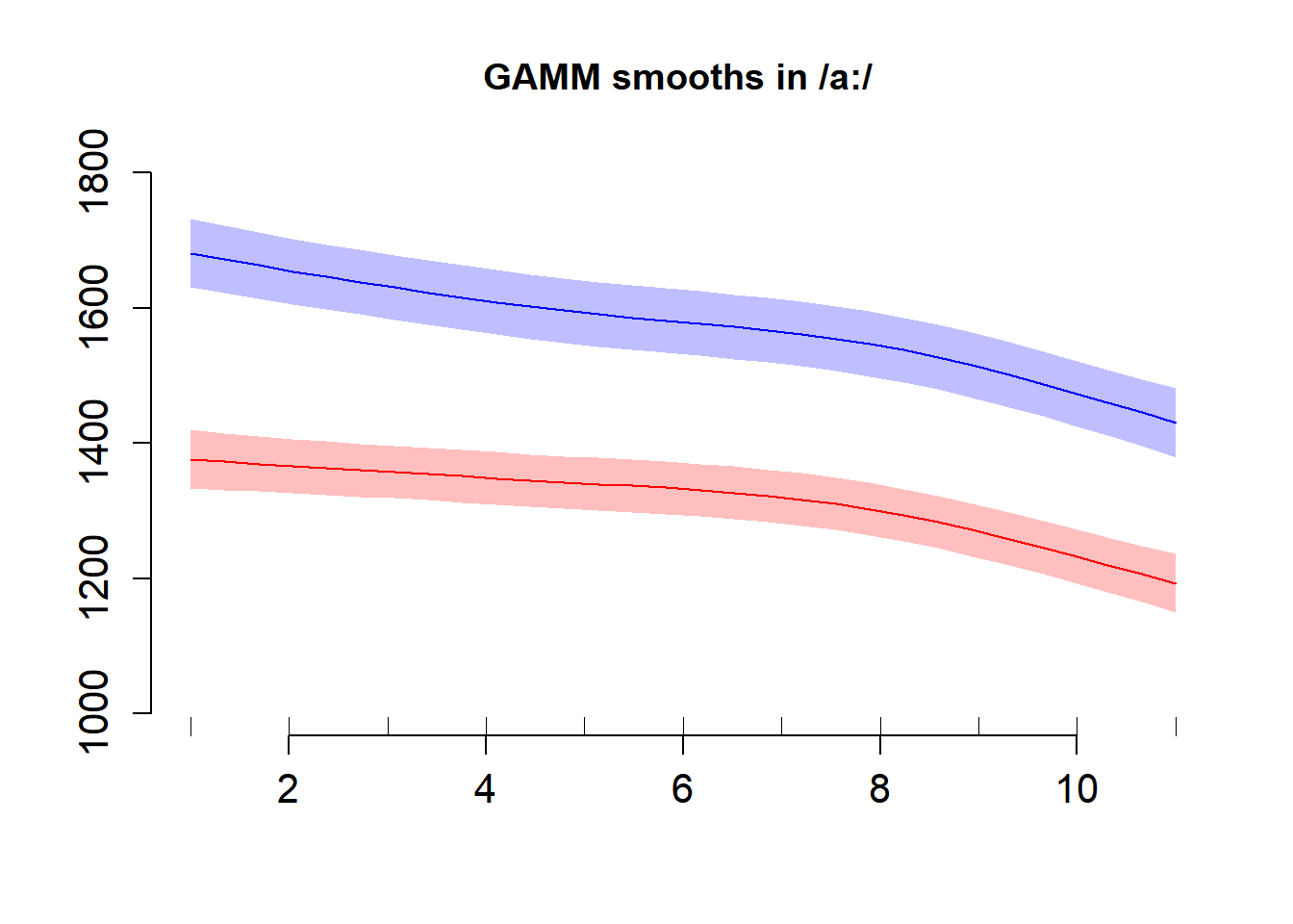

## Summary:
##  * ContVowInt.ord : factor; set to the value(s): Pharyngealised.a:. 
##  * Sex.ord : factor; set to the value(s): Female. 
##  * Interval : numeric predictor; with 30 values ranging from 1.000000 to 11.000000. 
##  * Speaker : factor; set to the value(s): SP01. (Might be canceled as random effect, check below.) 
##  * Word : factor; set to the value(s): 2aataa. (Might be canceled as random effect, check below.) 
##  * NOTE : The following random effects columns are canceled: s(Interval,Speaker),s(Interval,Speaker):ContVowInt.ordPlain.a:,s(Interval,Speaker):ContVowInt.ordPharyngealised.i:,s(Interval,Speaker):ContVowInt.ordPlain.i:,s(Interval,Speaker):ContVowInt.ordPharyngealised.u:,s(Interval,Speaker):ContVowInt.ordPlain.u:,s(Interval,Word),s(Interval,Word):Sex.ordMale
##  
## Note: Selection of grouping predictors does not seem to appear in data. Rug of all data is being added.

4.6.5.3 /u:/

plot_smooth(mdl.gamm.F2.AR, view = "Interval", cond = list(ContVowInt.ord = "Plain.u:"), col = "blue", ylab = "", xlab = "", main = "GAMM smooths in /u:/ ", hide.label = TRUE, cex.axis = 1.3, ylim = c(700, 1500), rm.ranef = TRUE)

## Summary:
##  * ContVowInt.ord : factor; set to the value(s): Plain.u:. 
##  * Sex.ord : factor; set to the value(s): Female. 
##  * Interval : numeric predictor; with 30 values ranging from 1.000000 to 11.000000. 
##  * Speaker : factor; set to the value(s): SP01. (Might be canceled as random effect, check below.) 
##  * Word : factor; set to the value(s): 2aataa. (Might be canceled as random effect, check below.) 
##  * NOTE : The following random effects columns are canceled: s(Interval,Speaker),s(Interval,Speaker):ContVowInt.ordPlain.a:,s(Interval,Speaker):ContVowInt.ordPharyngealised.i:,s(Interval,Speaker):ContVowInt.ordPlain.i:,s(Interval,Speaker):ContVowInt.ordPharyngealised.u:,s(Interval,Speaker):ContVowInt.ordPlain.u:,s(Interval,Word),s(Interval,Word):Sex.ordMale
## 

## Note: Selection of grouping predictors does not seem to appear in data. Rug of all data is being added.

plot_smooth(mdl.gamm.F2.AR, view = "Interval", cond = list(ContVowInt.ord = "Pharyngealised.u:"), col = "red", ylab = "", xlab = "", hide.label = TRUE, cex.axis = 1.3, ylim = c(700, 1500), rm.ranef = TRUE, add = TRUE)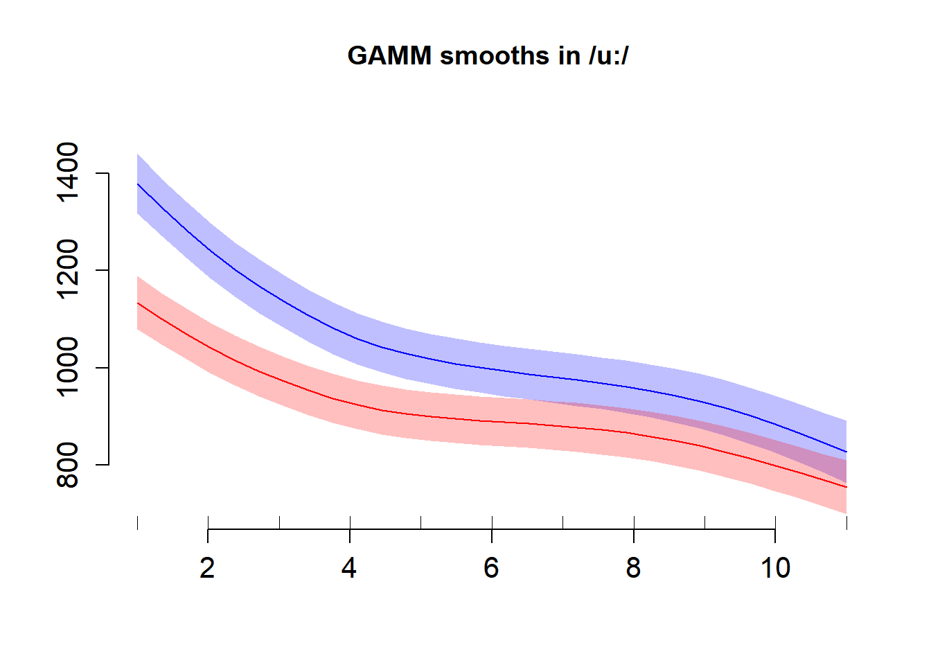

## Summary:
##  * ContVowInt.ord : factor; set to the value(s): Pharyngealised.u:. 
##  * Sex.ord : factor; set to the value(s): Female. 
##  * Interval : numeric predictor; with 30 values ranging from 1.000000 to 11.000000. 
##  * Speaker : factor; set to the value(s): SP01. (Might be canceled as random effect, check below.) 
##  * Word : factor; set to the value(s): 2aataa. (Might be canceled as random effect, check below.) 
##  * NOTE : The following random effects columns are canceled: s(Interval,Speaker),s(Interval,Speaker):ContVowInt.ordPlain.a:,s(Interval,Speaker):ContVowInt.ordPharyngealised.i:,s(Interval,Speaker):ContVowInt.ordPlain.i:,s(Interval,Speaker):ContVowInt.ordPharyngealised.u:,s(Interval,Speaker):ContVowInt.ordPlain.u:,s(Interval,Word),s(Interval,Word):Sex.ordMale
##  
## Note: Selection of grouping predictors does not seem to appear in data. Rug of all data is being added.

4.6.6 Difference smooths

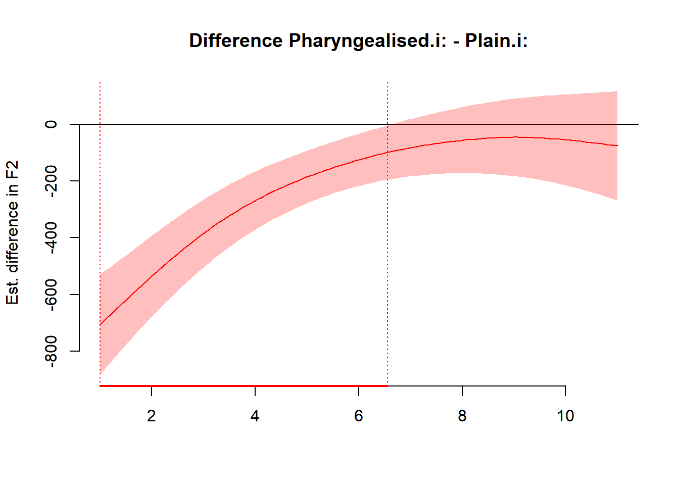
4.6.6.1 /i:/

plot_diff(mdl.gamm.F2.AR, view = "Interval", comp = list(ContVowInt.ord = c("Pharyngealised.i:","Plain.i:")),
          xlab = "",
          col = 'red', mark.diff =  TRUE, col.diff = "red",
          hide.label = TRUE, rm.ranef = TRUE)

## Summary:
##  * Sex.ord : factor; set to the value(s): Female. 
##  * Interval : numeric predictor; with 100 values ranging from 1.000000 to 11.000000. 
##  * Speaker : factor; set to the value(s): SP01. (Might be canceled as random effect, check below.) 
##  * Word : factor; set to the value(s): 2aataa. (Might be canceled as random effect, check below.) 
##  * NOTE : The following random effects columns are canceled: s(Interval,Speaker),s(Interval,Speaker):ContVowInt.ordPlain.a:,s(Interval,Speaker):ContVowInt.ordPharyngealised.i:,s(Interval,Speaker):ContVowInt.ordPlain.i:,s(Interval,Speaker):ContVowInt.ordPharyngealised.u:,s(Interval,Speaker):ContVowInt.ordPlain.u:,s(Interval,Word),s(Interval,Word):Sex.ordMale
## 

## 
## Interval window(s) of significant difference(s):
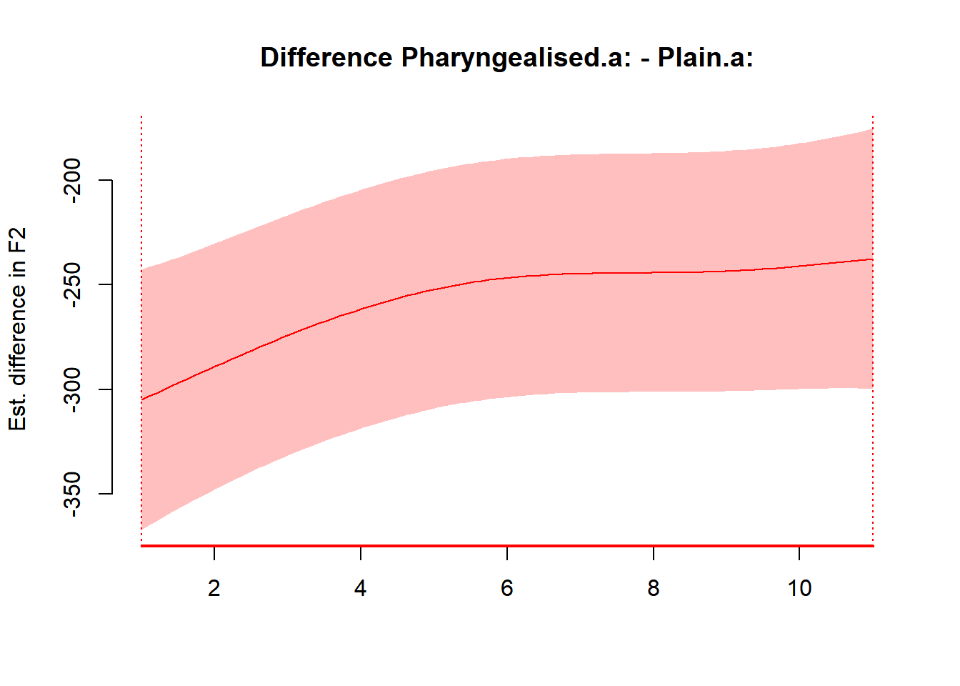
##  1.000000 - 6.555556

4.6.6.2 /a:/

plot_diff(mdl.gamm.F2.AR, view = "Interval", comp = list(ContVowInt.ord = c("Pharyngealised.a:","Plain.a:")),
          xlab = "",
          col = 'red', mark.diff =  TRUE, col.diff = "red",
          hide.label = TRUE, rm.ranef = TRUE)

## Summary:
##  * Sex.ord : factor; set to the value(s): Female. 
##  * Interval : numeric predictor; with 100 values ranging from 1.000000 to 11.000000. 
##  * Speaker : factor; set to the value(s): SP01. (Might be canceled as random effect, check below.) 
##  * Word : factor; set to the value(s): 2aataa. (Might be canceled as random effect, check below.) 
##  * NOTE : The following random effects columns are canceled: s(Interval,Speaker),s(Interval,Speaker):ContVowInt.ordPlain.a:,s(Interval,Speaker):ContVowInt.ordPharyngealised.i:,s(Interval,Speaker):ContVowInt.ordPlain.i:,s(Interval,Speaker):ContVowInt.ordPharyngealised.u:,s(Interval,Speaker):ContVowInt.ordPlain.u:,s(Interval,Word),s(Interval,Word):Sex.ordMale
## 

## 
## Interval window(s) of significant difference(s):
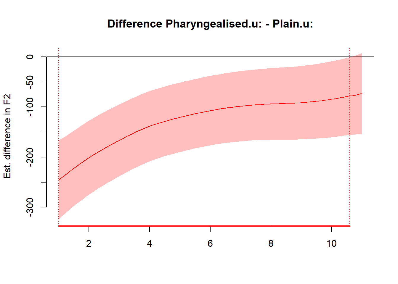
##  1.000000 - 11.000000

4.6.6.3 /u:/

plot_diff(mdl.gamm.F2.AR, view = "Interval", comp = list(ContVowInt.ord = c("Pharyngealised.u:","Plain.u:")),
          xlab = "",
          col = 'red', mark.diff =  TRUE, col.diff = "red",
          hide.label = TRUE, rm.ranef = TRUE)

## Summary:
##  * Sex.ord : factor; set to the value(s): Female. 
##  * Interval : numeric predictor; with 100 values ranging from 1.000000 to 11.000000. 
##  * Speaker : factor; set to the value(s): SP01. (Might be canceled as random effect, check below.) 
##  * Word : factor; set to the value(s): 2aataa. (Might be canceled as random effect, check below.) 
##  * NOTE : The following random effects columns are canceled: s(Interval,Speaker),s(Interval,Speaker):ContVowInt.ordPlain.a:,s(Interval,Speaker):ContVowInt.ordPharyngealised.i:,s(Interval,Speaker):ContVowInt.ordPlain.i:,s(Interval,Speaker):ContVowInt.ordPharyngealised.u:,s(Interval,Speaker):ContVowInt.ordPlain.u:,s(Interval,Word),s(Interval,Word):Sex.ordMale
## 

## 
## Interval window(s) of significant difference(s):
##  1.000000 - 10.595960