7.8 Multiple webpages
7.8.1 Read_html
## {html_document}
## <html>
## [1] <head>\n<meta http-equiv="Content-Type" content="text/html; charset=UTF-8 ...
## [2] <body>\n <div id="appTidyverseSite" class="shrinkHeader alwaysShrinkHead ...## {xml_nodeset (9)}
## [1] <a href="https://ggplot2.tidyverse.org/" target="_blank">\n <img class ...
## [2] <a href="https://dplyr.tidyverse.org/" target="_blank">\n <img class=" ...
## [3] <a href="https://tidyr.tidyverse.org/" target="_blank">\n <img class=" ...
## [4] <a href="https://readr.tidyverse.org/" target="_blank">\n <img class=" ...
## [5] <a href="https://purrr.tidyverse.org/" target="_blank">\n <img class=" ...
## [6] <a href="https://tibble.tidyverse.org/" target="_blank">\n <img class= ...
## [7] <a href="https://stringr.tidyverse.org/" target="_blank">\n <img class ...
## [8] <a href="https://forcats.tidyverse.org/" target="_blank">\n <img class ...
## [9] <a href="https://lubridate.tidyverse.org/" target="_blank">\n <img cla ...7.8.2 Extract headline
## [1] "https://ggplot2.tidyverse.org/"   "https://dplyr.tidyverse.org/"
## [3] "https://tidyr.tidyverse.org/"     "https://readr.tidyverse.org/"
## [5] "https://purrr.tidyverse.org/"     "https://tibble.tidyverse.org/"
## [7] "https://stringr.tidyverse.org/"   "https://forcats.tidyverse.org/"
## [9] "https://lubridate.tidyverse.org/"
7.8.3 Extract subpages
## [[1]]
## {html_document}
## <html lang="en">
## [1] <head>\n<meta http-equiv="Content-Type" content="text/html; charset=UTF-8 ...
## [2] <body>\n    <a href="#container" class="visually-hidden-focusable">Skip t ...
##
## [[2]]
## {html_document}
## <html lang="en">
## [1] <head>\n<meta http-equiv="Content-Type" content="text/html; charset=UTF-8 ...
## [2] <body>\n    <a href="#container" class="visually-hidden-focusable">Skip t ...
##
## [[3]]
## {html_document}
## <html lang="en">
## [1] <head>\n<meta http-equiv="Content-Type" content="text/html; charset=UTF-8 ...
## [2] <body>\n    <a href="#container" class="visually-hidden-focusable">Skip t ...
##
## [[4]]
## {html_document}
## <html lang="en">
## [1] <head>\n<meta http-equiv="Content-Type" content="text/html; charset=UTF-8 ...
## [2] <body>\n    <a href="#container" class="visually-hidden-focusable">Skip t ...
##
## [[5]]
## {html_document}
## <html lang="en">
## [1] <head>\n<meta http-equiv="Content-Type" content="text/html; charset=UTF-8 ...
## [2] <body>\n    <a href="#container" class="visually-hidden-focusable">Skip t ...
##
## [[6]]
## {html_document}
## <html lang="en">
## [1] <head>\n<meta http-equiv="Content-Type" content="text/html; charset=UTF-8 ...
## [2] <body>\n    <a href="#container" class="visually-hidden-focusable">Skip t ...
##
## [[7]]
## {html_document}
## <html lang="en">
## [1] <head>\n<meta http-equiv="Content-Type" content="text/html; charset=UTF-8 ...
## [2] <body>\n    <a href="#container" class="visually-hidden-focusable">Skip t ...
##
## [[8]]
## {html_document}
## <html lang="en">
## [1] <head>\n<meta http-equiv="Content-Type" content="text/html; charset=UTF-8 ...
## [2] <body>\n    <a href="#container" class="visually-hidden-focusable">Skip t ...
##
## [[9]]
## {html_document}
## <html lang="en">
## [1] <head>\n<meta http-equiv="Content-Type" content="text/html; charset=UTF-8 ...
## [2] <body>\n    <a href="#container" class="visually-hidden-focusable">Skip t ...
The structure seems to be similar across all pages
## [1] "ggplot2"   "dplyr"     "tidyr"     "readr"     "purrr"     "tibble"
## [7] "stringr"   "forcats"   "lubridate"
and extracting version number
pages %>%
  map(rvest::html_element, css = "small.nav-text.text-muted.me-auto") %>%
  map_chr(rvest::html_text)
## [1] "3.5.2" "1.1.4" "1.3.1" "2.1.5" "1.1.0" "3.3.0" "1.5.1" "1.0.0" "1.9.4"and we can also add all into a tibble
7.8.4 Extract text
pages_table <- tibble(
  name = pages %>%
    map(rvest::html_element, css = "a.navbar-brand") %>%
    map_chr(rvest::html_text),
  version = pages %>%
    map(rvest::html_element, css = "small.nav-text.text-muted.me-auto") %>%
    map_chr(rvest::html_text),
  CRAN = pages %>%
    map(rvest::html_element, css = "ul.list-unstyled > li:nth-child(1) > a") %>%
    map_chr(rvest::html_attr, name = "href"),
  Learn = pages %>%
    map(rvest::html_element, css = "ul.list-unstyled > li:nth-child(4) > a") %>%
    map_chr(rvest::html_attr, name = "href"),
  text = pages %>%
    map(rvest::html_element,  css = "body") %>%
    map_chr(rvest::html_text2)
)
pages_table
## # A tibble: 9 × 5
## name version CRAN Learn text
## <chr> <chr> <chr> <chr> <chr>
## 1 ggplot2 3.5.2 https://cloud.r-project.org/package=ggplot2 https:/… "Ski…
## 2 dplyr 1.1.4 https://cloud.r-project.org/package=dplyr http://… "Ski…
## 3 tidyr 1.3.1 https://cloud.r-project.org/package=tidyr https:/… "Ski…
## 4 readr 2.1.5 https://cloud.r-project.org/package=readr http://… "Ski…
## 5 purrr 1.1.0 https://cloud.r-project.org/package=purrr http://… "Ski…
## 6 tibble 3.3.0 https://cloud.r-project.org/package=tibble https:/… "Ski…
## 7 stringr 1.5.1 https://cloud.r-project.org/package=stringr http://… "Ski…
## 8 forcats 1.0.0 https://cloud.r-project.org/package=forcats http://… "Ski…
## 9 lubridate 1.9.4 https://cloud.r-project.org/package=lubridate https:/… "Ski…7.8.5 Create a corpus
## Corpus consisting of 9 documents and 4 docvars.
## text1 :
## "Skip to content ggplot23.5.2 Get started Reference News Rele..."
##
## text2 :
## "Skip to content dplyr1.1.4 Get started Reference Articles Gr..."
##
## text3 :
## "Skip to content tidyr1.3.1 Tidy data Reference Articles Pivo..."
##
## text4 :
## "Skip to content readr2.1.5 Get started Reference Articles Co..."
##
## text5 :
## "Skip to content purrr1.1.0 Reference Articles purrr <-> base..."
##
## text6 :
## "Skip to content tibble3.3.0 Get started Reference Articles C..."
##
## [ reached max_ndoc ... 3 more documents ]
7.8.5.1 Summary
## Corpus consisting of 9 documents, showing 9 documents:
##
##   Text Types Tokens Sentences      name version
##  text1   368    777        24   ggplot2   3.5.2
##  text2   419   1258        17     dplyr   1.1.4
##  text3   326    729        25     tidyr   1.3.1
##  text4   571   1745        47     readr   2.1.5
##  text5   248    495        11     purrr   1.1.0
##  text6   269    717        14    tibble   3.3.0
##  text7   398   1345        23   stringr   1.5.1
##  text8   264    648        14   forcats   1.0.0
##  text9   267    650        11 lubridate   1.9.4
##                                           CRAN
##    https://cloud.r-project.org/package=ggplot2
##      https://cloud.r-project.org/package=dplyr
##      https://cloud.r-project.org/package=tidyr
##      https://cloud.r-project.org/package=readr
##      https://cloud.r-project.org/package=purrr
##     https://cloud.r-project.org/package=tibble
##    https://cloud.r-project.org/package=stringr
##    https://cloud.r-project.org/package=forcats
##  https://cloud.r-project.org/package=lubridate
##                                           Learn
##  https://r4ds.had.co.nz/data-visualisation.html
##            http://r4ds.had.co.nz/transform.html
##                https://r4ds.hadley.nz/data-tidy
##          http://r4ds.had.co.nz/data-import.html
##            http://r4ds.had.co.nz/iteration.html
##             https://r4ds.had.co.nz/tibbles.html
##              http://r4ds.hadley.nz/strings.html
##              http://r4ds.had.co.nz/factors.html
##           https://r4ds.hadley.nz/datetimes.html
7.8.5.2 Accessing parts of corpus
## [1] "Skip to content\nreadr2.1.5\nGet started\nReference\nArticles\nColumn type Locales\nNews\nReleases\nVersion 2.1.0Version 2.0.0Version 1.4.0Version 1.3.1Version 1.0.0Version 0.2.0Version 0.1.0\nChangelog\nreadr\nOverview\n\nThe goal of readr is to provide a fast and friendly way to read rectangular data from delimited files, such as comma-separated values (CSV) and tab-separated values (TSV). It is designed to parse many types of data found in the wild, while providing an informative problem report when parsing leads to unexpected results. If you are new to readr, the best place to start is the data import chapter in R for Data Science.\n\nInstallation\n\n# The easiest way to get readr is to install the whole tidyverse:\ninstall.packages(\"tidyverse\")\n\n# Alternatively, install just readr:\ninstall.packages(\"readr\")\nCheatsheet\n\nUsage\n\nreadr is part of the core tidyverse, so you can load it with:\n\n\nlibrary(tidyverse)\n#> ── Attaching core tidyverse packages ──────────────────────── tidyverse 2.0.0 ──\n#> ✔ dplyr 1.1.4 ✔ readr 2.1.4.9000\n#> ✔ forcats 1.0.0 ✔ stringr 1.5.1 \n#> ✔ ggplot2 3.4.3 ✔ tibble 3.2.1 \n#> ✔ lubridate 1.9.3 ✔ tidyr 1.3.0 \n#> ✔ purrr 1.0.2 \n#> ── Conflicts ────────────────────────────────────────── tidyverse_conflicts() ──\n#> ✖ dplyr::filter() masks stats::filter()\n#> ✖ dplyr::lag() masks stats::lag()\n#> ℹ Use the conflicted package (<http://conflicted.r-lib.org/>) to force all conflicts to become errors\n\nOf course, you can also load readr as an individual package:\n\n\nlibrary(readr)\n\nTo read a rectangular dataset with readr, you combine two pieces: a function that parses the lines of the file into individual fields and a column specification.\n\nreadr supports the following file formats with these read_*() functions:\n\nread_csv(): comma-separated values (CSV)\nread_tsv(): tab-separated values (TSV)\nread_csv2(): semicolon-separated values with , as the decimal mark\nread_delim(): delimited files (CSV and TSV are important special cases)\nread_fwf(): fixed-width files\nread_table(): whitespace-separated files\nread_log(): web log files\n\nA column specification describes how each column should be converted from a character vector to a specific data type (e.g. character, numeric, datetime, etc.). In the absence of a column specification, readr will guess column types from the data. vignette(\"column-types\") gives more detail on how readr guesses the column types. Column type guessing is very handy, especially during data exploration, but it’s important to remember these are just guesses. As any data analysis project matures past the exploratory phase, the best strategy is to provide explicit column types.\n\nThe following example loads a sample file bundled with readr and guesses the column types:\n\n\n(chickens <- read_csv(readr_example(\"chickens.csv\")))\n#> Rows: 5 Columns: 4\n#> ── Column specification ────────────────────────────────────────────────────────\n#> Delimiter: \",\"\n#> chr (3): chicken, sex, motto\n#> dbl (1): eggs_laid\n#> \n#> ℹ Use `spec()` to retrieve the full column specification for this data.\n#> ℹ Specify the column types or set `show_col_types = FALSE` to quiet this message.\n#> # A tibble: 5 × 4\n#> chicken sex eggs_laid motto \n#> <chr> <chr> <dbl> <chr> \n#> 1 Foghorn Leghorn rooster 0 That's a joke, ah say, that's a jok…\n#> 2 Chicken Little hen 3 The sky is falling! \n#> 3 Ginger hen 12 Listen. We'll either die free chick…\n#> 4 Camilla the Chicken hen 7 Bawk, buck, ba-gawk. \n#> 5 Ernie The Giant Chicken rooster 0 Put Captain Solo in the cargo hold.\n\nNote that readr prints the column types – the guessed column types, in this case. This is useful because it allows you to check that the columns have been read in as you expect. If they haven’t, that means you need to provide the column specification. This sounds like a lot of trouble, but luckily readr affords a nice workflow for this. Use spec() to retrieve the (guessed) column specification from your initial effort.\n\n\nspec(chickens)\n#> cols(\n#> chicken = col_character(),\n#> sex = col_character(),\n#> eggs_laid = col_double(),\n#> motto = col_character()\n#> )\n\nNow you can copy, paste, and tweak this, to create a more explicit readr call that expresses the desired column types. Here we express that sex should be a factor with levels rooster and hen, in that order, and that eggs_laid should be integer.\n\n\nchickens <- read_csv(\n readr_example(\"chickens.csv\"),\n col_types = cols(\n chicken = col_character(),\n sex = col_factor(levels = c(\"rooster\", \"hen\")),\n eggs_laid = col_integer(),\n motto = col_character()\n )\n)\nchickens\n#> # A tibble: 5 × 4\n#> chicken sex eggs_laid motto \n#> <chr> <fct> <int> <chr> \n#> 1 Foghorn Leghorn rooster 0 That's a joke, ah say, that's a jok…\n#> 2 Chicken Little hen 3 The sky is falling! \n#> 3 Ginger hen 12 Listen. We'll either die free chick…\n#> 4 Camilla the Chicken hen 7 Bawk, buck, ba-gawk. \n#> 5 Ernie The Giant Chicken rooster 0 Put Captain Solo in the cargo hold.\n\nvignette(\"readr\") gives an expanded introduction to readr.\n\nEditions\n\nreadr got a new parsing engine in version 2.0.0 (released July 2021). In this so-called second edition, readr calls vroom::vroom(), by default.\n\nThe parsing engine in readr versions prior to 2.0.0 is now called the first edition. If you’re using readr >= 2.0.0, you can still access first edition parsing via the functions with_edition(1, ...) and local_edition(1). And, obviously, if you’re using readr < 2.0.0, you will get first edition parsing, by definition, because that’s all there is.\n\nWe will continue to support the first edition for a number of releases, but the overall goal is to make the second edition uniformly better than the first. Therefore the plan is to eventually deprecate and then remove the first edition code. New code and actively-maintained code should use the second edition. The workarounds with_edition(1, ...) and local_edition(1) are offered as a pragmatic way to patch up legacy code or as a temporary solution for infelicities identified as the second edition matures.\n\nAlternatives\n\nThere are two main alternatives to readr: base R and data.table’s fread(). The most important differences are discussed below.\n\nBase R\n\nCompared to the corresponding base functions, readr functions:\n\nUse a consistent naming scheme for the parameters (e.g. col_names and col_types not header and colClasses).\n\nAre generally much faster (up to 10x-100x) depending on the dataset.\n\nLeave strings as is by default, and automatically parse common date/time formats.\n\nHave a helpful progress bar if loading is going to take a while.\n\nAll functions work exactly the same way regardless of the current locale. To override the US-centric defaults, use locale().\n\ndata.table and fread()\n\ndata.table has a function similar to read_csv() called fread(). Compared to fread(), readr functions:\n\nAre sometimes slower, particularly on numeric heavy data.\n\nCan automatically guess some parameters, but basically encourage explicit specification of, e.g., the delimiter, skipped rows, and the header row.\n\nFollow tidyverse-wide conventions, such as returning a tibble, a standard approach for column name repair, and a common mini-language for column selection.\n\nAcknowledgements\n\nThanks to:\n\nJoe Cheng for showing me the beauty of deterministic finite automata for parsing, and for teaching me why I should write a tokenizer.\n\nJJ Allaire for helping me come up with a design that makes very few copies, and is easy to extend.\n\nDirk Eddelbuettel for coming up with the name!\n\nLinks\nView on CRAN\nBrowse source code\nReport a bug\nLearn more\nLicense\nFull license\nMIT + file LICENSE\nCommunity\nContributing guide\nCode of conduct\nGetting help\nCitation\nCiting readr\nDevelopers\nHadley Wickham\nAuthor\nJim Hester\nAuthor\nJennifer Bryan\nAuthor, maintainer\n\nCopyright holder, funder\nMore about authors...\n\nDeveloped by Hadley Wickham, Jim Hester, Jennifer Bryan, .\n\nSite built with pkgdown 2.0.7."7.8.5.3 Document-level information
##      name version                                        CRAN
## 1 ggplot2   3.5.2 https://cloud.r-project.org/package=ggplot2
## 2   dplyr   1.1.4   https://cloud.r-project.org/package=dplyr
## 3   tidyr   1.3.1   https://cloud.r-project.org/package=tidyr
## 4   readr   2.1.5   https://cloud.r-project.org/package=readr
## 5   purrr   1.1.0   https://cloud.r-project.org/package=purrr
## 6  tibble   3.3.0  https://cloud.r-project.org/package=tibble
##                                            Learn
## 1 https://r4ds.had.co.nz/data-visualisation.html
## 2           http://r4ds.had.co.nz/transform.html
## 3               https://r4ds.hadley.nz/data-tidy
## 4         http://r4ds.had.co.nz/data-import.html
## 5           http://r4ds.had.co.nz/iteration.html
## 6            https://r4ds.had.co.nz/tibbles.html
7.8.6 Tokens
tokens() segments texts in a corpus into tokens (words or sentences) by word boundaries.
We can remove punctuations or not
7.8.6.1 With punctuations
## Tokens consisting of 9 documents and 4 docvars.
## text1 :
##  [1] "Skip"         "to"           "content"      "ggplot23.5.2" "Get"
##  [6] "started"      "Reference"    "News"         "Releases"     "Version"
## [11] "3.5.0"        "Version"
## [ ... and 765 more ]
##
## text2 :
##  [1] "Skip"       "to"         "content"    "dplyr1.1.4" "Get"
##  [6] "started"    "Reference"  "Articles"   "Grouped"    "data"
## [11] "Two-table"  "verbs"
## [ ... and 1,246 more ]
##
## text3 :
##  [1] "Skip"        "to"          "content"     "tidyr1.3.1"  "Tidy"
##  [6] "data"        "Reference"   "Articles"    "Pivoting"    "Rectangling"
## [11] "Nested"      "data"
## [ ... and 717 more ]
##
## text4 :
##  [1] "Skip"       "to"         "content"    "readr2.1.5" "Get"
##  [6] "started"    "Reference"  "Articles"   "Column"     "type"
## [11] "Locales"    "News"
## [ ... and 1,733 more ]
##
## text5 :
##  [1] "Skip"       "to"         "content"    "purrr1.1.0" "Reference"
##  [6] "Articles"   "purrr"      "<"          "-"          ">"
## [11] "base"       "R"
## [ ... and 483 more ]
##
## text6 :
##  [1] "Skip"        "to"          "content"     "tibble3.3.0" "Get"
##  [6] "started"     "Reference"   "Articles"    "Column"      "types"
## [11] "Controlling" "display"
## [ ... and 705 more ]
##
## [ reached max_ndoc ... 3 more documents ]
7.8.6.2 Without punctuations
web_pages_txt_corpus_tok_no_punct <- tokens(web_pages_txt_corpus, remove_punct = TRUE)
web_pages_txt_corpus_tok_no_punct
## Tokens consisting of 9 documents and 4 docvars.
## text1 :
## [1] "Skip" "to" "content" "ggplot23.5.2" "Get"
## [6] "started" "Reference" "News" "Releases" "Version"
## [11] "3.5.0" "Version"
## [ ... and 635 more ]
##
## text2 :
## [1] "Skip" "to" "content" "dplyr1.1.4" "Get"
## [6] "started" "Reference" "Articles" "Grouped" "data"
## [11] "Two-table" "verbs"
## [ ... and 988 more ]
##
## text3 :
## [1] "Skip" "to" "content" "tidyr1.3.1" "Tidy"
## [6] "data" "Reference" "Articles" "Pivoting" "Rectangling"
## [11] "Nested" "data"
## [ ... and 547 more ]
##
## text4 :
## [1] "Skip" "to" "content" "readr2.1.5" "Get"
## [6] "started" "Reference" "Articles" "Column" "type"
## [11] "Locales" "News"
## [ ... and 1,364 more ]
##
## text5 :
## [1] "Skip" "to" "content" "purrr1.1.0" "Reference"
## [6] "Articles" "purrr" "<" ">" "base"
## [11] "R" "Functional"
## [ ... and 376 more ]
##
## text6 :
## [1] "Skip" "to" "content" "tibble3.3.0" "Get"
## [6] "started" "Reference" "Articles" "Column" "types"
## [11] "Controlling" "display"
## [ ... and 536 more ]
##
## [ reached max_ndoc ... 3 more documents ]7.8.7 Stop words
It is best to remove stop words (function/grammatical words) when we use statistical analyses of a corpus.
web_pages_txt_corpus_tok_no_punct_no_Stop <- tokens_select(web_pages_txt_corpus_tok_no_punct, pattern = stopwords("en", source = "stopwords-iso"), selection = "remove")
web_pages_txt_corpus_tok_no_punct_no_Stop
## Tokens consisting of 9 documents and 4 docvars.
## text1 :
## [1] "Skip" "content" "ggplot23.5.2" "started" "Reference"
## [6] "News" "Releases" "Version" "3.5.0" "Version"
## [11] "3.4.0" "Version"
## [ ... and 339 more ]
##
## text2 :
## [1] "Skip" "content" "dplyr1.1.4" "started" "Reference"
## [6] "Articles" "data" "Two-table" "verbs" "dplyr"
## [11] "<" ">"
## [ ... and 733 more ]
##
## text3 :
## [1] "Skip" "content" "tidyr1.3.1" "Tidy" "data"
## [6] "Reference" "Articles" "Pivoting" "Rectangling" "Nested"
## [11] "data" "articles"
## [ ... and 322 more ]
##
## text4 :
## [1] "Skip" "content" "readr2.1.5" "started" "Reference"
## [6] "Articles" "Column" "type" "Locales" "News"
## [11] "Releases" "Version"
## [ ... and 884 more ]
##
## text5 :
## [1] "Skip" "content" "purrr1.1.0" "Reference" "Articles"
## [6] "purrr" "<" ">" "base" "Functional"
## [11] "programming" "languages"
## [ ... and 227 more ]
##
## text6 :
## [1] "Skip" "content" "tibble3.3.0" "started" "Reference"
## [6] "Articles" "Column" "types" "Controlling" "display"
## [11] "Comparing" "display"
## [ ... and 338 more ]
##
## [ reached max_ndoc ... 3 more documents ]7.8.8 Statistical analyses
We can start by providing statistics (whether descriptives or inferential) based on our corpora.
7.8.8.1 Simple frequency analysis
Here we look at obtaining a simple frequency analysis of usage.
7.8.8.1.1 DFM
We start by generating a DFM (document-feature matrix)
web_pages_txt_corpus_tok_no_punct_no_Stop_dfm <- dfm(web_pages_txt_corpus_tok_no_punct_no_Stop)
web_pages_txt_corpus_tok_no_punct_no_Stop_dfm
## Document-feature matrix of: 9 documents, 1,182 features (81.12% sparse) and 4 docvars.
## features
## docs skip content ggplot23.5.2 started reference news releases version 3.5.0
## text1 1 1 1 1 1 1 1 11 1
## text2 1 1 0 1 1 1 1 10 0
## text3 1 1 0 1 1 1 1 13 0
## text4 1 1 0 1 1 1 2 2 0
## text5 1 1 0 0 1 1 1 5 0
## text6 1 1 0 1 1 1 1 7 0
## features
## docs 3.4.0
## text1 1
## text2 0
## text3 0
## text4 0
## text5 0
## text6 0
## [ reached max_ndoc ... 3 more documents, reached max_nfeat ... 1,172 more features ]7.8.8.1.2 Frequencies
web_pages_txt_corpus_tok_no_punct_no_Stop_dfm_freq <- textstat_frequency(web_pages_txt_corpus_tok_no_punct_no_Stop_dfm)
web_pages_txt_corpus_tok_no_punct_no_Stop_dfm_freq
## feature frequency rank docfreq group
## 1 > 271 1 7 all
## 2 ─ 132 2 1 all
## 3 < 91 3 8 all
## 4 1 72 4 6 all
## 5 version 55 5 9 all
## 6 data 55 5 9 all
## 7 2 47 7 7 all
## 8 3 39 8 5 all
## 9 = 38 9 8 all
## 10 tidyverse 33 10 9 all
## 11 code 32 11 9 all
## 12 tibble 32 11 4 all
## 13 chr 31 13 4 all
## 14 author 30 14 9 all
## 15 readr 29 15 1 all
## 16 ggplot2 28 16 3 all
## 17 functions 28 16 7 all
## 18 column 28 16 3 all
## 19 install.packages 26 19 9 all
## 20 license 26 19 9 all
## 21 4 25 21 7 all
## 22 5 23 22 5 all
## 23 dplyr 22 23 3 all
## 24 learn 20 24 9 all
## 25 install 19 25 9 all
## 26 pak 18 26 6 all
## 27 hadley 18 26 9 all
## 28 wickham 18 26 9 all
## 29 time 18 26 5 all
## 30 + 16 30 8 all
## 31 tidyr 16 30 2 all
## 32 library 14 32 9 all
## 33 file 14 32 8 all
## 34 values 14 32 4 all
## 35 stringr 14 32 2 all
## 36 purrr 14 32 2 all
## 37 bug 13 37 9 all
## 38 conduct 13 37 9 all
## 39 species 13 37 2 all
## 40 dbl 13 37 3 all
## 41 types 12 41 3 all
## 42 × 12 41 4 all
## 43 forcats 12 41 2 all
## 44 lubridate 12 41 2 all
## 45 start 11 45 8 all
## 46 community 11 45 9 all
## 47 vignette 11 45 6 all
## 48 ℹ 11 45 3 all
## 49 chicken 11 45 1 all
## 50 releases 10 50 9 all
## 51 articles 10 50 7 all
## 52 github 10 50 7 all
## 53 list 10 50 3 all
## 54 source 10 50 9 all
## 55 report 10 50 9 all
## 56 contributing 10 50 8 all
## 57 built 10 50 9 all
## 58 mass 10 50 1 all
## 59 aeiou 10 50 1 all
## 60 pattern 10 50 1 all
## 61 skip 9 61 9 all
## 62 content 9 61 9 all
## 63 started 9 61 8 all
## 64 reference 9 61 9 all
## 65 news 9 61 9 all
## 66 1.0.0 9 61 6 all
## 67 changelog 9 61 9 all
## 68 overview 9 61 9 all
## 69 map 9 61 2 all
## 70 variables 9 61 4 all
## 71 installation 9 61 9 all
## 72 easiest 9 61 9 all
## 73 alternatively 9 61 9 all
## 74 development 9 61 7 all
## 75 science 9 61 8 all
## 76 common 9 61 5 all
## 77 set 9 61 7 all
## 78 links 9 61 9 all
## 79 view 9 61 9 all
## 80 cran 9 61 9 all
## 81 browse 9 61 9 all
## 82 guide 9 61 8 all
## 83 citation 9 61 9 all
## 84 citing 9 61 9 all
## 85 developers 9 61 9 all
## 86 maintainer 9 61 9 all
## 87 copyright 9 61 8 all
## 88 holder 9 61 8 all
## 89 developed 9 61 9 all
## 90 pkgdown 9 61 9 all
## 91 base 9 61 4 all
## 92 starwars 9 61 2 all
## 93 true 9 61 4 all
## 94 specification 9 61 2 all
## 95 ✔ 9 61 1 all
## 96 edition 9 61 1 all
## 97 mit 8 97 8 all
## 98 funder 8 97 8 all
## 99 rows 8 97 3 all
## 100 6 8 97 4 all
## 101 sex 8 97 2 all
## 102 red 8 97 1 all
## 103 character 8 97 5 all
## 104 hen 8 97 1 all
## 105 string 8 97 1 all
## 106 30 8 97 1 all
## 107 2.0.0 7 107 3 all
## 108 faq 7 107 1 all
## 109 graphics 7 107 1 all
## 110 cheatsheet 7 107 7 all
## 111 read 7 107 5 all
## 112 filter 7 107 3 all
## 113 chapter 7 107 7 all
## 114 data.table 7 107 4 all
## 115 eye_color 7 107 2 all
## 116 project 7 107 4 all
## 117 tidy 7 107 1 all
## 118 type 7 107 4 all
## 119 parsing 7 107 2 all
## 120 strings 7 107 2 all
## 121 match 7 107 1 all
## 122 factors 7 107 1 all
## 123 provide 6 123 4 all
## 124 usage 6 123 6 all
## 125 lionel 6 123 3 all
## 126 henry 6 123 3 all
## 127 operations 6 123 3 all
## 128 multiple 6 123 4 all
## 129 single 6 123 3 all
## 130 tibbles 6 123 3 all
## 131 datasets 6 123 2 all
## 132 columns 6 123 3 all
## 133 missing 6 123 2 all
## 134 eggs_laid 6 123 1 all
## 135 rooster 6 123 1 all
## 136 0 6 123 2 all
## 137 inputs 6 123 2 all
## 138 regular 6 123 1 all
## 139 create 5 139 4 all
## 140 questions 5 139 4 all
## 141 verbs 5 139 2 all
## 142 names 5 139 3 all
## 143 extra 5 139 2 all
## 144 white 5 139 1 all
## 145 blue 5 139 1 all
## 146 15 5 139 2 all
## 147 row 5 139 3 all
## 148 brown 5 139 1 all
## 149 mascu 5 139 1 all
## 150 variable 5 139 3 all
## 151 explicit 5 139 2 all
## 152 package 5 139 4 all
## 153 files 5 139 1 all
## 154 e.g 5 139 2 all
## 155 motto 5 139 1 all
## 156 col_character 5 139 1 all
## 157 factor 5 139 2 all
## 158 levels 5 139 3 all
## 159 easy 5 139 3 all
## 160 vectors 5 139 3 all
## 161 argument 5 139 2 all
## 162 expressions 5 139 1 all
## 163 devtools 5 139 2 all
## 164 bday 5 139 1 all
## 165 reordering 4 165 2 all
## 166 details 4 165 2 all
## 167 ggplot 4 165 2 all
## 168 aes 4 165 2 all
## 169 existing 4 165 3 all
## 170 designed 4 165 4 all
## 171 thomas 4 165 2 all
## 172 recommend 4 165 3 all
## 173 solve 4 165 4 all
## 174 pieces 4 165 4 all
## 175 main 4 165 4 all
## 176 reproducible 4 165 4 all
## 177 2.1.3 4 165 4 all
## 178 programming 4 165 3 all
## 179 consistent 4 165 4 all
## 180 mutate 4 165 2 all
## 181 summary 4 165 3 all
## 182 droid 4 165 2 all
## 183 height 4 165 1 all
## 184 yellow 4 165 1 all
## 185 masculi 4 165 1 all
## 186 human 4 165 3 all
## 187 note 4 165 4 all
## 188 released 4 165 4 all
## 189 kirill 4 165 2 all
## 190 müller 4 165 2 all
## 191 davis 4 165 2 all
## 192 vaughan 4 165 2 all
## 193 goal 4 165 3 all
## 194 pivot 4 165 1 all
## 195 authors 4 165 4 all
## 196 function 4 165 2 all
## 197 read_csv 4 165 1 all
## 198 vector 4 165 3 all
## 199 chickens 4 165 1 all
## 200 ` 4 165 1 all
## 201 you’re 4 165 3 all
## 202 fread 4 165 1 all
## 203 extract 4 165 2 all
## 204 | 4 165 1 all
## 205 ~ 4 165 2 all
## 206 components 4 165 3 all
## 207 easily 4 165 2 all
## 208 matching 4 165 2 all
## 209 letters 4 165 2 all
## 210 stringi 4 165 1 all
## 211 video 4 165 1 all
## 212 cross 4 165 1 all
## 213 deal 4 165 1 all
## 214 authority 4 165 1 all
## 215 addin 4 165 1 all
## 216 date-time 4 165 1 all
## 217 date-times 4 165 1 all
## 218 2010-12-13 4 165 1 all
## 219 packages 3 219 3 all
## 220 performance 3 219 2 all
## 221 ✨ 3 219 3 all
## 222 based 3 219 2 all
## 223 hard 3 219 2 all
## 224 dataset 3 219 2 all
## 225 coord_flip 3 219 2 all
## 226 changing 3 219 2 all
## 227 introduction 3 219 2 all
## 228 individual 3 219 2 all
## 229 you’d 3 219 2 all
## 230 kara 3 219 1 all
## 231 woo 3 219 1 all
## 232 lin 3 219 1 all
## 233 pedersen 3 219 1 all
## 234 winston 3 219 1 all
## 235 chang 3 219 1 all
## 236 you’ve 3 219 3 all
## 237 analysis 3 219 3 all
## 238 describes 3 219 3 all
## 239 fit 3 219 3 all
## 240 rstudio 3 219 2 all
## 241 friendly 3 219 3 all
## 242 two-table 3 219 1 all
## 243 1.1.0 3 219 3 all
## 244 manipulation 3 219 2 all
## 245 providing 3 219 3 all
## 246 select 3 219 1 all
## 247 combine 3 219 3 all
## 248 backends 3 219 1 all
## 249 frames 3 219 2 all
## 250 engine 3 219 2 all
## 251 translates 3 219 1 all
## 252 duckdb 3 219 1 all
## 253 14 3 219 2 all
## 254 hair_color 3 219 1 all
## 255 skin_color 3 219 1 all
## 256 c-3po 3 219 1 all
## 257 r2-d2 3 219 1 all
## 258 96 3 219 1 all
## 259 32 3 219 1 all
## 260 87 3 219 1 all
## 261 darth 3 219 1 all
## 262 82 3 219 1 all
## 263 bmi 3 219 1 all
## 264 136 3 219 1 all
## 265 male 3 219 1 all
## 266 9 3 219 3 all
## 267 gungan 3 219 2 all
## 268 35 3 219 2 all
## 269 encounter 3 219 3 all
## 270 minimal 3 219 3 all
## 271 discussion 3 219 3 all
## 272 community.rstudio.com 3 219 3 all
## 273 contributor 3 219 3 all
## 274 agree 3 219 3 all
## 275 abide 3 219 3 all
## 276 terms 3 219 3 all
## 277 nested 3 219 1 all
## 278 0.1.0 3 219 3 all
## 279 tools 3 219 3 all
## 280 spread 3 219 2 all
## 281 lists 3 219 3 all
## 282 frame 3 219 3 all
## 283 reshape 3 219 1 all
## 284 interactive 3 219 2 all
## 285 fast 3 219 3 all
## 286 csv 3 219 1 all
## 287 tsv 3 219 1 all
## 288 core 3 219 2 all
## 289 load 3 219 2 all
## 290 lag 3 219 2 all
## 291 formats 3 219 2 all
## 292 numeric 3 219 2 all
## 293 guesses 3 219 1 all
## 294 spec 3 219 1 all
## 295 false 3 219 3 all
## 296 7 3 219 2 all
## 297 default 3 219 2 all
## 298 compared 3 219 2 all
## 299 progress 3 219 2 all
## 300 2.0.7 3 219 3 all
## 301 languages 3 219 2 all
## 302 easier 3 219 3 all
## 303 display 3 219 2 all
## 304 data.frame 3 219 1 all
## 305 don’t 3 219 2 all
## 306 change 3 219 2 all
## 307 patterns 3 219 1 all
## 308 str_subset 3 219 1 all
## 309 str_count 3 219 1 all
## 310 extracts 3 219 1 all
## 311 outputs 3 219 1 all
## 312 categorical 3 219 1 all
## 313 leap 3 219 1 all
## 314 times 3 219 1 all
## 315 sun 3 219 1 all
## 316 fri 3 219 1 all
## 317 3.0.0 2 317 2 all
## 318 aesthetic 2 317 1 all
## 319 specifications 2 317 1 all
## 320 developer 2 317 2 all
## 321 extending 2 317 2 all
## 322 faceting 2 317 1 all
## 323 grammar 2 317 2 all
## 324 it’s 2 317 2 all
## 325 add 2 317 1 all
## 326 geom_point 2 317 1 all
## 327 mpg 2 317 2 all
## 328 behaviour 2 317 1 all
## 329 extensions 2 317 1 all
## 330 reading 2 317 2 all
## 331 visualization 2 317 1 all
## 332 chapters 2 317 1 all
## 333 comprehensive 2 317 2 all
## 334 follow 2 317 2 all
## 335 mastered 2 317 2 all
## 336 illustrates 2 317 2 all
## 337 kohske 2 317 1 all
## 338 takahashi 2 317 1 all
## 339 claus 2 317 1 all
## 340 wilke 2 317 1 all
## 341 hiroaki 2 317 1 all
## 342 yutani 2 317 1 all
## 343 dewey 2 317 1 all
## 344 dunnington 2 317 1 all
## 345 teun 2 317 1 all
## 346 van 2 317 1 all
## 347 den 2 317 1 all
## 348 brand 2 317 1 all
## 349 0.8.0 2 317 2 all
## 350 picks 2 317 1 all
## 351 summarise 2 317 1 all
## 352 arrange 2 317 1 all
## 353 naturally 2 317 2 all
## 354 group_by 2 317 1 all
## 355 transformation 2 317 2 all
## 356 arrow 2 317 1 all
## 357 including 2 317 2 all
## 358 apache 2 317 1 all
## 359 in-memory 2 317 1 all
## 360 stored 2 317 1 all
## 361 database 2 317 2 all
## 362 sql 2 317 2 all
## 363 copies 2 317 2 all
## 364 translation 2 317 2 all
## 365 birth_year 2 317 1 all
## 366 gender 2 317 1 all
## 367 167 2 317 1 all
## 368 75 2 317 1 all
## 369 gold 2 317 1 all
## 370 ig-88 2 317 1 all
## 371 200 2 317 1 all
## 372 140 2 317 1 all
## 373 metal 2 317 1 all
## 374 homeworld 2 317 1 all
## 375 films 2 317 1 all
## 376 vehicles 2 317 1 all
## 377 starships 2 317 1 all
## 378 luke 2 317 1 all
## 379 skywalker 2 317 1 all
## 380 vader 2 317 1 all
## 381 leia 2 317 1 all
## 382 organa 2 317 1 all
## 383 light 2 317 2 all
## 384 ^ 2 317 2 all
## 385 202 2 317 1 all
## 386 wh 2 317 2 all
## 387 kaminoan 2 317 2 all
## 388 mirialan 2 317 2 all
## 389 romain 2 317 1 all
## 390 françois 2 317 1 all
## 391 pivoting 2 317 1 all
## 392 rectangling 2 317 1 all
## 393 1.3.0 2 317 2 all
## 394 1.2.0 2 317 2 all
## 395 0.3.0 2 317 2 all
## 396 observation 2 317 1 all
## 397 cell 2 317 1 all
## 398 standard 2 317 2 all
## 399 converts 2 317 1 all
## 400 introduces 2 317 2 all
## 401 gather 2 317 1 all
## 402 nest 2 317 1 all
## 403 implicit 2 317 1 all
## 404 complete 2 317 2 all
## 405 replace 2 317 2 all
## 406 reshape2 2 317 1 all
## 407 iteration 2 317 2 all
## 408 reshaping 2 317 1 all
## 409 implementations 2 317 2 all
## 410 melt 2 317 1 all
## 411 cleaning 2 317 2 all
## 412 maximilian 2 317 1 all
## 413 girlich 2 317 1 all
## 414 1.4.0version 2 317 2 all
## 415 1.0.0version 2 317 2 all
## 416 0.2.0version 2 317 2 all
## 417 rectangular 2 317 1 all
## 418 delimited 2 317 1 all
## 419 comma-separated 2 317 1 all
## 420 tab-separated 2 317 1 all
## 421 parse 2 317 1 all
## 422 conflicts 2 317 1 all
## 423 ✖ 2 317 1 all
## 424 masks 2 317 1 all
## 425 stats 2 317 1 all
## 426 guess 2 317 1 all
## 427 matures 2 317 1 all
## 428 readr_example 2 317 1 all
## 429 chickens.csv 2 317 1 all
## 430 delimiter 2 317 1 all
## 431 retrieve 2 317 1 all
## 432 foghorn 2 317 1 all
## 433 leghorn 2 317 1 all
## 434 joke 2 317 1 all
## 435 jok 2 317 1 all
## 436 sky 2 317 1 all
## 437 falling 2 317 1 all
## 438 ginger 2 317 1 all
## 439 12 2 317 1 all
## 440 listen 2 317 1 all
## 441 die 2 317 1 all
## 442 chick 2 317 1 all
## 443 camilla 2 317 1 all
## 444 bawk 2 317 1 all
## 445 buck 2 317 1 all
## 446 ba-gawk 2 317 1 all
## 447 ernie 2 317 1 all
## 448 giant 2 317 1 all
## 449 captain 2 317 1 all
## 450 solo 2 317 1 all
## 451 cargo 2 317 1 all
## 452 hold 2 317 1 all
## 453 guessed 2 317 1 all
## 454 check 2 317 2 all
## 455 cols 2 317 1 all
## 456 col_types 2 317 1 all
## 457 fct 2 317 2 all
## 458 vroom 2 317 1 all
## 459 called 2 317 1 all
## 460 with_edition 2 317 1 all
## 461 local_edition 2 317 1 all
## 462 alternatives 2 317 1 all
## 463 parameters 2 317 1 all
## 464 header 2 317 1 all
## 465 depending 2 317 2 all
## 466 automatically 2 317 1 all
## 467 helpful 2 317 2 all
## 468 locale 2 317 1 all
## 469 conventions 2 317 2 all
## 470 jim 2 317 1 all
## 471 hester 2 317 1 all
## 472 jennifer 2 317 1 all
## 473 bryan 2 317 1 all
## 474 functional 2 317 1 all
## 475 fp 2 317 1 all
## 476 split 2 317 1 all
## 477 mtcars 2 317 1 all
## 478 df 2 317 1 all
## 479 map_dbl 2 317 1 all
## 480 8 2 317 2 all
## 481 advantages 2 317 1 all
## 482 pipe 2 317 2 all
## 483 output 2 317 2 all
## 484 returns 2 317 1 all
## 485 position 2 317 2 all
## 486 track 2 317 2 all
## 487 comparing 2 317 1 all
## 488 data.frames 2 317 1 all
## 489 print 2 317 1 all
## 490 method 2 317 1 all
## 491 objects 2 317 2 all
## 492 object 2 317 2 all
## 493 as_tibble 2 317 1 all
## 494 2025-03-18 2 317 1 all
## 495 2025-03-17 2 317 1 all
## 496 2025-03-16 2 317 1 all
## 497 17 2 317 2 all
## 498 features 2 317 2 all
## 499 tribble 2 317 1 all
## 500 3.6 2 317 1 all
## 501 8.5 2 317 1 all
## 502 doesn’t 2 317 1 all
## 503 str_c 2 317 1 all
## 504 matches 2 317 1 all
## 505 vowel 2 317 1 all
## 506 str_detect 2 317 1 all
## 507 str_locate 2 317 1 all
## 508 str_extract 2 317 1 all
## 509 str_match 2 317 1 all
## 510 str_replace 2 317 1 all
## 511 str_split 2 317 1 all
## 512 fixed 2 317 2 all
## 513 exact 2 317 2 all
## 514 regexplain 2 317 1 all
## 515 resources 2 317 2 all
## 516 install_github 2 317 2 all
## 517 result 2 317 1 all
## 518 fct_infreq 2 317 1 all
## 519 fct_lump 2 317 1 all
## 520 is.na 2 317 1 all
## 521 count 2 317 1 all
## 522 geom_bar 2 317 1 all
## 523 stringsasfactors 2 317 1 all
## 524 zones 2 317 1 all
## 525 savings 2 317 1 all
## 526 ymd 2 317 1 all
## 527 ymd_hms 2 317 1 all
## 528 dmy 2 317 1 all
## 529 mdy 2 317 1 all
## 530 month 2 317 1 all
## 531 wday 2 317 1 all
## 532 label 2 317 1 all
## 533 mon 2 317 1 all
## 534 tue 2 317 1 all
## 535 thu 2 317 1 all
## 536 sat 2 317 1 all
## 537 with_tz 2 317 1 all
## 538 force_tz 2 317 1 all
## 539 america 2 317 1 all
## 540 chicago 2 317 1 all
## 541 cst 2 317 1 all
## 542 vitalie 2 317 1 all
## 543 spinu 2 317 1 all
## 544 garrett 2 317 1 all
## 545 grolemund 2 317 1 all
## 546 ggplot23.5.2 1 546 1 all
## 547 3.5.0 1 546 1 all
## 548 3.4.0 1 546 1 all
## 549 3.3.0 1 546 1 all
## 550 3.2.0 1 546 1 all
## 551 3.1.0 1 546 1 all
## 552 2.2.0 1 546 1 all
## 553 2.1.0 1 546 1 all
## 554 profiling 1 546 1 all
## 555 axes 1 546 1 all
## 556 customising 1 546 1 all
## 557 annotation 1 546 1 all
## 558 barplots 1 546 1 all
## 559 declaratively 1 546 1 all
## 560 creating 1 546 1 all
## 561 aesthetics 1 546 1 all
## 562 graphical 1 546 1 all
## 563 primitives 1 546 1 all
## 564 takes 1 546 1 all
## 565 care 1 546 1 all
## 566 succinctly 1 546 1 all
## 567 embodies 1 546 1 all
## 568 deep 1 546 1 all
## 569 philosophy 1 546 1 all
## 570 visualisation 1 546 1 all
## 571 supply 1 546 1 all
## 572 mapping 1 546 1 all
## 573 layers 1 546 1 all
## 574 geom_histogram 1 546 1 all
## 575 scales 1 546 1 all
## 576 scale_colour_brewer 1 546 1 all
## 577 facet_wrap 1 546 1 all
## 578 coordinate 1 546 1 all
## 579 systems 1 546 1 all
## 580 displ 1 546 1 all
## 581 hwy 1 546 1 all
## 582 colour 1 546 1 all
## 583 class 1 546 1 all
## 584 lifecycle 1 546 1 all
## 585 hundreds 1 546 1 all
## 586 thousands 1 546 1 all
## 587 people 1 546 1 all
## 588 millions 1 546 1 all
## 589 plots 1 546 1 all
## 590 by-and-large 1 546 1 all
## 591 arguments 1 546 1 all
## 592 compelling 1 546 1 all
## 593 reasons 1 546 1 all
## 594 innovation 1 546 1 all
## 595 rich 1 546 1 all
## 596 ecosystem 1 546 1 all
## 597 maintained 1 546 1 all
## 598 https://exts.ggplot2.tidyverse.org/gallery/. 1 546 1 all
## 599 learning 1 546 1 all
## 600 starting 1 546 1 all
## 601 systematic 1 546 1 all
## 602 documentation 1 546 1 all
## 603 communication 1 546 1 all
## 604 speed 1 546 1 all
## 605 essentials 1 546 1 all
## 606 online 1 546 1 all
## 607 webinar 1 546 1 all
## 608 plotting 1 546 1 all
## 609 dive 1 546 1 all
## 610 cookbook 1 546 1 all
## 611 recipes 1 546 1 all
## 612 basics 1 546 1 all
## 613 elegant 1 546 1 all
## 614 theoretical 1 546 1 all
## 615 underpinnings 1 546 1 all
## 616 book 1 546 1 all
## 617 helps 1 546 1 all
## 618 understand 1 546 1 all
## 619 theory 1 546 1 all
## 620 underpins 1 546 1 all
## 621 tailored 1 546 1 all
## 622 stack 1 546 1 all
## 623 overflow 1 546 1 all
## 624 answers 1 546 1 all
## 625 created 1 546 1 all
## 626 🧩 1 546 1 all
## 627 dplyr1.1.4 1 546 1 all
## 628 automation 1 546 1 all
## 629 column-wise 1 546 1 all
## 630 row-wise 1 546 1 all
## 631 0.8.3 1 546 1 all
## 632 0.8.2 1 546 1 all
## 633 0.8.1 1 546 1 all
## 634 0.7.5 1 546 1 all
## 635 challenges 1 546 1 all
## 636 adds 1 546 1 all
## 637 reduces 1 546 1 all
## 638 perform 1 546 1 all
## 639 operation 1 546 1 all
## 640 single-table 1 546 1 all
## 641 variety 1 546 1 all
## 642 addition 1 546 1 all
## 643 computational 1 546 1 all
## 644 accessible 1 546 1 all
## 645 efficient 1 546 1 all
## 646 alternative 1 546 1 all
## 647 larger-than-memory 1 546 1 all
## 648 remote 1 546 1 all
## 649 cloud 1 546 1 all
## 650 storage 1 546 1 all
## 651 aws 1 546 1 all
## 652 s3 1 546 1 all
## 653 acero 1 546 1 all
## 654 dtplyr 1 546 1 all
## 655 dbplyr 1 546 1 all
## 656 relational 1 546 1 all
## 657 duckplyr 1 546 1 all
## 658 queries 1 546 1 all
## 659 automatic 1 546 1 all
## 660 fallback 1 546 1 all
## 661 isn’t 1 546 1 all
## 662 sparklyr 1 546 1 all
## 663 spark 1 546 1 all
## 664 feature 1 546 1 all
## 665 cheat 1 546 1 all
## 666 sheet 1 546 1 all
## 667 112 1 546 1 all
## 668 33 1 546 1 all
## 669 r5-d4 1 546 1 all
## 670 97 1 546 1 all
## 671 r4-p17 1 546 1 all
## 672 silver 1 546 1 all
## 673 feminine 1 546 1 all
## 674 ends_with 1 546 1 all
## 675 color 1 546 1 all
## 676 blond 1 546 1 all
## 677 fair 1 546 1 all
## 678 100 1 546 1 all
## 679 172 1 546 1 all
## 680 77 1 546 1 all
## 681 26.0 1 546 1 all
## 682 26.9 1 546 1 all
## 683 34.7 1 546 1 all
## 684 33.3 1 546 1 all
## 685 150 1 546 1 all
## 686 49 1 546 1 all
## 687 21.8 1 546 1 all
## 688 desc 1 546 1 all
## 689 jabba 1 546 1 all
## 690 175 1 546 1 all
## 691 1358 1 546 1 all
## 692 green-tan 1 546 1 all
## 693 orange 1 546 1 all
## 694 600 1 546 1 all
## 695 herm 1 546 1 all
## 696 grievous 1 546 1 all
## 697 216 1 546 1 all
## 698 159 1 546 1 all
## 699 green 1 546 1 all
## 700 41.9 1 546 1 all
## 701 tarfful 1 546 1 all
## 702 234 1 546 1 all
## 703 na.rm 1 546 1 all
## 704 50 1 546 1 all
## 705 69.8 1 546 1 all
## 706 74 1 546 1 all
## 707 81.3 1 546 1 all
## 708 88 1 546 1 all
## 709 53.1 1 546 1 all
## 710 issue 1 546 1 all
## 711 manipulatr 1 546 1 all
## 712 mailing 1 546 1 all
## 713 participating 1 546 1 all
## 714 tidyr1.3.1 1 546 1 all
## 715 0.7.0 1 546 1 all
## 716 0.6.0 1 546 1 all
## 717 0.5.0 1 546 1 all
## 718 0.4.0 1 546 1 all
## 719 0.2.0 1 546 1 all
## 720 storing 1 546 1 all
## 721 ensure 1 546 1 all
## 722 you’ll 1 546 1 all
## 723 spend 1 546 1 all
## 724 fighting 1 546 1 all
## 725 tidy-data 1 546 1 all
## 726 fall 1 546 1 all
## 727 categories 1 546 1 all
## 728 wide 1 546 1 all
## 729 forms 1 546 1 all
## 730 pivot_longer 1 546 1 all
## 731 pivot_wider 1 546 1 all
## 732 replacing 1 546 1 all
## 733 deeply 1 546 1 all
## 734 json 1 546 1 all
## 735 unnest_longer 1 546 1 all
## 736 unnest_wider 1 546 1 all
## 737 hoist 1 546 1 all
## 738 rectangle 1 546 1 all
## 739 nesting 1 546 1 all
## 740 form 1 546 1 all
## 741 unnesting 1 546 1 all
## 742 unnest 1 546 1 all
## 743 splitting 1 546 1 all
## 744 combining 1 546 1 all
## 745 separate_wider_delim 1 546 1 all
## 746 separate_wider_position 1 546 1 all
## 747 separate_wider_regex 1 546 1 all
## 748 pull 1 546 1 all
## 749 unite 1 546 1 all
## 750 drop_na 1 546 1 all
## 751 previous 1 546 1 all
## 752 replace_na 1 546 1 all
## 753 supersedes 1 546 1 all
## 754 2010-2014 1 546 1 all
## 755 2005-2010 1 546 1 all
## 756 counterintuitively 1 546 1 all
## 757 tidying 1 546 1 all
## 758 aggregation 1 546 1 all
## 759 high-performance 1 546 1 all
## 760 dcast 1 546 1 all
## 761 perspective 1 546 1 all
## 762 i’d 1 546 1 all
## 763 papers 1 546 1 all
## 764 wrangler 1 546 1 all
## 765 visual 1 546 1 all
## 766 scripts 1 546 1 all
## 767 framework 1 546 1 all
## 768 potter’s 1 546 1 all
## 769 wheel 1 546 1 all
## 770 efficiently 1 546 1 all
## 771 implementing 1 546 1 all
## 772 schemasql 1 546 1 all
## 773 here’s 1 546 1 all
## 774 terminology 1 546 1 all
## 775 wider 1 546 1 all
## 776 cast 1 546 1 all
## 777 spreadsheets 1 546 1 all
## 778 unpivot 1 546 1 all
## 779 databases 1 546 1 all
## 780 fold 1 546 1 all
## 781 unfold 1 546 1 all
## 782 readr2.1.5 1 546 1 all
## 783 locales 1 546 1 all
## 784 2.1.0version 1 546 1 all
## 785 2.0.0version 1 546 1 all
## 786 1.3.1version 1 546 1 all
## 787 wild 1 546 1 all
## 788 informative 1 546 1 all
## 789 leads 1 546 1 all
## 790 unexpected 1 546 1 all
## 791 import 1 546 1 all
## 792 attaching 1 546 1 all
## 793 1.1.4 1 546 1 all
## 794 2.1.4.9000 1 546 1 all
## 795 1.5.1 1 546 1 all
## 796 3.4.3 1 546 1 all
## 797 3.2.1 1 546 1 all
## 798 1.9.3 1 546 1 all
## 799 1.0.2 1 546 1 all
## 800 tidyverse_conflicts 1 546 1 all
## 801 conflicted 1 546 1 all
## 802 http://conflicted.r-lib.org/ 1 546 1 all
## 803 force 1 546 1 all
## 804 errors 1 546 1 all
## 805 parses 1 546 1 all
## 806 lines 1 546 1 all
## 807 fields 1 546 1 all
## 808 supports 1 546 1 all
## 809 read_ 1 546 1 all
## 810 read_tsv 1 546 1 all
## 811 read_csv2 1 546 1 all
## 812 semicolon-separated 1 546 1 all
## 813 decimal 1 546 1 all
## 814 mark 1 546 1 all
## 815 read_delim 1 546 1 all
## 816 special 1 546 1 all
## 817 read_fwf 1 546 1 all
## 818 fixed-width 1 546 1 all
## 819 read_table 1 546 1 all
## 820 whitespace-separated 1 546 1 all
## 821 read_log 1 546 1 all
## 822 log 1 546 1 all
## 823 converted 1 546 1 all
## 824 specific 1 546 1 all
## 825 datetime 1 546 1 all
## 826 absence 1 546 1 all
## 827 column-types 1 546 1 all
## 828 guessing 1 546 1 all
## 829 handy 1 546 1 all
## 830 exploration 1 546 1 all
## 831 remember 1 546 1 all
## 832 exploratory 1 546 1 all
## 833 phase 1 546 1 all
## 834 strategy 1 546 1 all
## 835 loads 1 546 1 all
## 836 sample 1 546 1 all
## 837 bundled 1 546 1 all
## 838 show_col_types 1 546 1 all
## 839 quiet 1 546 1 all
## 840 message 1 546 1 all
## 841 prints 1 546 1 all
## 842 expect 1 546 1 all
## 843 haven’t 1 546 1 all
## 844 sounds 1 546 1 all
## 845 lot 1 546 1 all
## 846 trouble 1 546 1 all
## 847 luckily 1 546 1 all
## 848 affords 1 546 1 all
## 849 nice 1 546 1 all
## 850 workflow 1 546 1 all
## 851 initial 1 546 1 all
## 852 effort 1 546 1 all
## 853 col_double 1 546 1 all
## 854 paste 1 546 1 all
## 855 tweak 1 546 1 all
## 856 expresses 1 546 1 all
## 857 desired 1 546 1 all
## 858 express 1 546 1 all
## 859 integer 1 546 1 all
## 860 col_factor 1 546 1 all
## 861 col_integer 1 546 1 all
## 862 expanded 1 546 1 all
## 863 editions 1 546 1 all
## 864 july 1 546 1 all
## 865 2021 1 546 1 all
## 866 so-called 1 546 1 all
## 867 calls 1 546 1 all
## 868 versions 1 546 1 all
## 869 prior 1 546 1 all
## 870 access 1 546 1 all
## 871 definition 1 546 1 all
## 872 that’s 1 546 1 all
## 873 continue 1 546 1 all
## 874 support 1 546 1 all
## 875 uniformly 1 546 1 all
## 876 plan 1 546 1 all
## 877 eventually 1 546 1 all
## 878 deprecate 1 546 1 all
## 879 remove 1 546 1 all
## 880 actively-maintained 1 546 1 all
## 881 workarounds 1 546 1 all
## 882 offered 1 546 1 all
## 883 pragmatic 1 546 1 all
## 884 patch 1 546 1 all
## 885 legacy 1 546 1 all
## 886 temporary 1 546 1 all
## 887 solution 1 546 1 all
## 888 infelicities 1 546 1 all
## 889 identified 1 546 1 all
## 890 data.table’s 1 546 1 all
## 891 differences 1 546 1 all
## 892 discussed 1 546 1 all
## 893 naming 1 546 1 all
## 894 scheme 1 546 1 all
## 895 col_names 1 546 1 all
## 896 colclasses 1 546 1 all
## 897 faster 1 546 1 all
## 898 10x-100x 1 546 1 all
## 899 leave 1 546 1 all
## 900 bar 1 546 1 all
## 901 loading 1 546 1 all
## 902 current 1 546 1 all
## 903 override 1 546 1 all
## 904 us-centric 1 546 1 all
## 905 defaults 1 546 1 all
## 906 slower 1 546 1 all
## 907 heavy 1 546 1 all
## 908 basically 1 546 1 all
## 909 encourage 1 546 1 all
## 910 skipped 1 546 1 all
## 911 tidyverse-wide 1 546 1 all
## 912 returning 1 546 1 all
## 913 approach 1 546 1 all
## 914 repair 1 546 1 all
## 915 mini-language 1 546 1 all
## 916 selection 1 546 1 all
## 917 acknowledgements 1 546 1 all
## 918 joe 1 546 1 all
## 919 cheng 1 546 1 all
## 920 beauty 1 546 1 all
## 921 deterministic 1 546 1 all
## 922 finite 1 546 1 all
## 923 automata 1 546 1 all
## 924 teaching 1 546 1 all
## 925 write 1 546 1 all
## 926 tokenizer 1 546 1 all
## 927 jj 1 546 1 all
## 928 allaire 1 546 1 all
## 929 helping 1 546 1 all
## 930 design 1 546 1 all
## 931 extend 1 546 1 all
## 932 dirk 1 546 1 all
## 933 eddelbuettel 1 546 1 all
## 934 coming 1 546 1 all
## 935 purrr1.1.0 1 546 1 all
## 936 0.2.3 1 546 1 all
## 937 enhances 1 546 1 all
## 938 r’s 1 546 1 all
## 939 toolkit 1 546 1 all
## 940 heard 1 546 1 all
## 941 family 1 546 1 all
## 942 loops 1 546 1 all
## 943 succinct 1 546 1 all
## 944 realistic 1 546 1 all
## 945 model 1 546 1 all
## 946 piece 1 546 1 all
## 947 compute 1 546 1 all
## 948 r2 1 546 1 all
## 949 $ 1 546 1 all
## 950 cyl 1 546 1 all
## 951 lm 1 546 1 all
## 952 wt 1 546 1 all
## 953 r.squared 1 546 1 all
## 954 0.5086326 1 546 1 all
## 955 0.4645102 1 546 1 all
## 956 0.4229655 1 546 1 all
## 957 equivalents 1 546 1 all
## 958 type-stable 1 546 1 all
## 959 return 1 546 1 all
## 960 advertised 1 546 1 all
## 961 double 1 546 1 all
## 962 throw 1 546 1 all
## 963 error 1 546 1 all
## 964 accept 1 546 1 all
## 965 named 1 546 1 all
## 966 anonymous 1 546 1 all
## 967 lambda 1 546 1 all
## 968 obvious 1 546 1 all
## 969 running 1 546 1 all
## 970 jobs 1 546 1 all
## 971 in_parallel 1 546 1 all
## 972 computation 1 546 1 all
## 973 cores 1 546 1 all
## 974 machines 1 546 1 all
## 975 network 1 546 1 all
## 976 tibble3.3.0 1 546 1 all
## 977 controlling 1 546 1 all
## 978 invariants 1 546 1 all
## 979 behavior 1 546 1 all
## 980 2.1.1 1 546 1 all
## 981 2.0.1 1 546 1 all
## 982 pre-announcement 1 546 1 all
## 983 1.4.2 1 546 1 all
## 984 1.4.1 1 546 1 all
## 985 tbl_df 1 546 1 all
## 986 modern 1 546 1 all
## 987 reimagining 1 546 1 all
## 988 keeping 1 546 1 all
## 989 proven 1 546 1 all
## 990 effective 1 546 1 all
## 991 throwing 1 546 1 all
## 992 lazy 1 546 1 all
## 993 surly 1 546 1 all
## 994 i.e 1 546 1 all
## 995 partial 1 546 1 all
## 996 complain 1 546 1 all
## 997 exist 1 546 1 all
## 998 forces 1 546 1 all
## 999 confront 1 546 1 all
## 1000 earlier 1 546 1 all
## 1001 typically 1 546 1 all
## 1002 leading 1 546 1 all
## 1003 cleaner 1 546 1 all
## 1004 expressive 1 546 1 all
## 1005 enhanced 1 546 1 all
## 1006 complex 1 546 1 all
## 1007 sys.date 1 546 1 all
## 1008 reasonable 1 546 1 all
## 1009 matrices 1 546 1 all
## 1010 tables 1 546 1 all
## 1011 26 1 546 1 all
## 1012 recycles 1 546 1 all
## 1013 creates 1 546 1 all
## 1014 row.names 1 546 1 all
## 1015 define 1 546 1 all
## 1016 row-by-row 1 546 1 all
## 1017 draws 1 546 1 all
## 1018 inspiration 1 546 1 all
## 1019 rownames 1 546 1 all
## 1020 2.1.3.9000 1 546 1 all
## 1021 stringr1.5.1 1 546 1 all
## 1022 1.5.0version 1 546 1 all
## 1023 1.3.0version 1 546 1 all
## 1024 1.2.0version 1 546 1 all
## 1025 1.1.0version 1 546 1 all
## 1026 glamorous 1 546 1 all
## 1027 high-profile 1 546 1 all
## 1028 play 1 546 1 all
## 1029 role 1 546 1 all
## 1030 preparation 1 546 1 all
## 1031 tasks 1 546 1 all
## 1032 cohesive 1 546 1 all
## 1033 familiar 1 546 1 all
## 1034 icu 1 546 1 all
## 1035 correct 1 546 1 all
## 1036 manipulations 1 546 1 all
## 1037 focusses 1 546 1 all
## 1038 commonly 1 546 1 all
## 1039 covering 1 546 1 all
## 1040 imagine 1 546 1 all
## 1041 share 1 546 1 all
## 1042 str_ 1 546 1 all
## 1043 str_length 1 546 1 all
## 1044 collapse 1 546 1 all
## 1045 str_sub 1 546 1 all
## 1046 concise 1 546 1 all
## 1047 language 1 546 1 all
## 1048 describing 1 546 1 all
## 1049 expression 1 546 1 all
## 1050 tells 1 546 1 all
## 1051 there’s 1 546 1 all
## 1052 counts 1 546 1 all
## 1053 defined 1 546 1 all
## 1054 parentheses 1 546 1 all
## 1055 characters 1 546 1 all
## 1056 vid 1 546 1 all
## 1057 ros 1 546 1 all
## 1058 dea 1 546 1 all
## 1059 aut 1 546 1 all
## 1060 replacement 1 546 1 all
## 1061 replaces 1 546 1 all
## 1062 deo 1 546 1 all
## 1063 ss 1 546 1 all
## 1064 xtra 1 546 1 all
## 1065 uthority 1 546 1 all
## 1066 splits 1 546 1 all
## 1067 engines 1 546 1 all
## 1068 bytes 1 546 1 all
## 1069 coll 1 546 1 all
## 1070 boundary 1 546 1 all
## 1071 boundaries 1 546 1 all
## 1072 interface 1 546 1 all
## 1073 interactively 1 546 1 all
## 1074 build 1 546 1 all
## 1075 regexp 1 546 1 all
## 1076 consult 1 546 1 all
## 1077 included 1 546 1 all
## 1078 installed 1 546 1 all
## 1079 gadenbuie 1 546 1 all
## 1080 solid 1 546 1 all
## 1081 grown 1 546 1 all
## 1082 organically 1 546 1 all
## 1083 inconsistent 1 546 1 all
## 1084 additionally 1 546 1 all
## 1085 ruby 1 546 1 all
## 1086 python 1 546 1 all
## 1087 modify 1 546 1 all
## 1088 conjunction 1 546 1 all
## 1089 str_pad 1 546 1 all
## 1090 11 1 546 1 all
## 1091 simplifies 1 546 1 all
## 1092 eliminating 1 546 1 all
## 1093 options 1 546 1 all
## 1094 95 1 546 1 all
## 1095 produces 1 546 1 all
## 1096 includes 1 546 1 all
## 1097 ensuring 1 546 1 all
## 1098 from-base 1 546 1 all
## 1099 r4ds 1 546 1 all
## 1100 forcats1.0.0 1 546 1 all
## 1101 0.5.0version 1 546 1 all
## 1102 0.4.0version 1 546 1 all
## 1103 0.3.0version 1 546 1 all
## 1104 handle 1 546 1 all
## 1105 improve 1 546 1 all
## 1106 suite 1 546 1 all
## 1107 examples 1 546 1 all
## 1108 include 1 546 1 all
## 1109 fct_reorder 1 546 1 all
## 1110 frequency 1 546 1 all
## 1111 fct_relevel 1 546 1 all
## 1112 hand 1 546 1 all
## 1113 collapsing 1 546 1 all
## 1114 frequent 1 546 1 all
## 1115 sort 1 546 1 all
## 1116 37 1 546 1 all
## 1117 twi'lek 1 546 1 all
## 1118 wookiee 1 546 1 all
## 1119 zabrak 1 546 1 all
## 1120 aleena 1 546 1 all
## 1121 besalisk 1 546 1 all
## 1122 27 1 546 1 all
## 1123 history 1 546 1 all
## 1124 unauthorized 1 546 1 all
## 1125 biography 1 546 1 all
## 1126 roger 1 546 1 all
## 1127 peng 1 546 1 all
## 1128 sigh 1 546 1 all
## 1129 lumley 1 546 1 all
## 1130 approaches 1 546 1 all
## 1131 wrangling 1 546 1 all
## 1132 amelia 1 546 1 all
## 1133 mcnamara 1 546 1 all
## 1134 nicholas 1 546 1 all
## 1135 horton 1 546 1 all
## 1136 lubridate1.9.4 1 546 1 all
## 1137 1.7.0 1 546 1 all
## 1138 1.6.0 1 546 1 all
## 1139 frustrating 1 546 1 all
## 1140 commands 1 546 1 all
## 1141 unintuitive 1 546 1 all
## 1142 methods 1 546 1 all
## 1143 robust 1 546 1 all
## 1144 days 1 546 1 all
## 1145 daylight 1 546 1 all
## 1146 quirks 1 546 1 all
## 1147 lacks 1 546 1 all
## 1148 capabilities 1 546 1 all
## 1149 situations 1 546 1 all
## 1150 warn.conflicts 1 546 1 all
## 1151 dmy_hms 1 546 1 all
## 1152 20101215 1 546 1 all
## 1153 2010-12-15 1 546 1 all
## 1154 2017-04-01 1 546 1 all
## 1155 simple 1 546 1 all
## 1156 mday 1 546 1 all
## 1157 hour 1 546 1 all
## 1158 minute 1 546 1 all
## 1159 1979 1 546 1 all
## 1160 2016 1 546 1 all
## 1161 helper 1 546 1 all
## 1162 handling 1 546 1 all
## 1163 utc 1 546 1 all
## 1164 printing 1 546 1 all
## 1165 09 1 546 1 all
## 1166 expands 1 546 1 all
## 1167 mathematical 1 546 1 all
## 1168 performed 1 546 1 all
## 1169 span 1 546 1 all
## 1170 classes 1 546 1 all
## 1171 borrowed 1 546 1 all
## 1172 https://www.joda.org 1 546 1 all
## 1173 durations 1 546 1 all
## 1174 measure 1 546 1 all
## 1175 periods 1 546 1 all
## 1176 accurately 1 546 1 all
## 1177 clock 1 546 1 all
## 1178 day 1 546 1 all
## 1179 intervals 1 546 1 all
## 1180 protean 1 546 1 all
## 1181 gpl 1 546 1 all
## 1182 2.1.2 1 546 1 all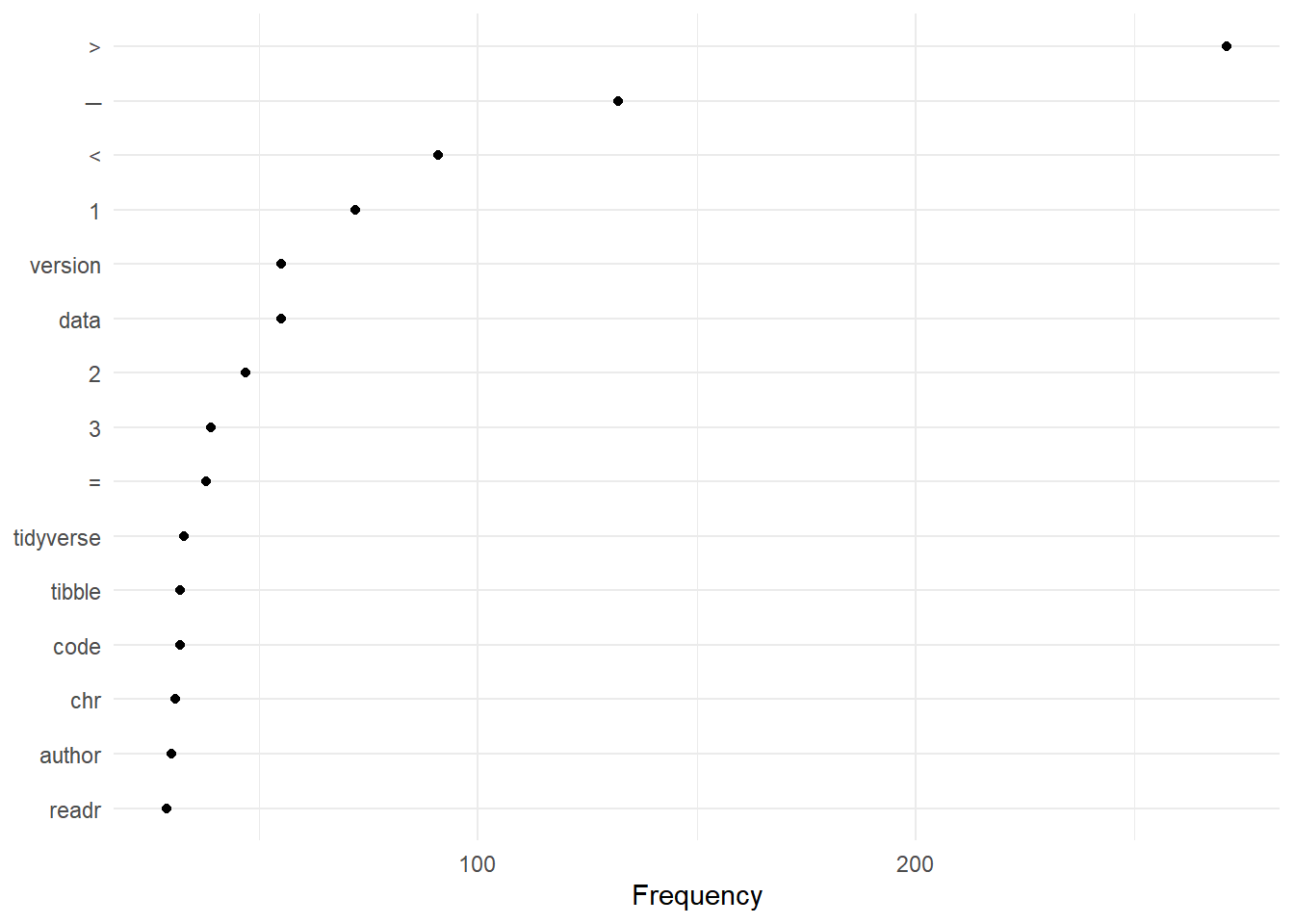
7.8.8.2 Lexical diversity
We can compute the lexical diversity in a document. This is a measure allowing us to provide a statistical account of diversity in the choice of lexical items in a text. See the different measures implemented here
7.8.8.2.1 TTR (Type-Token Ratio)
7.8.8.2.1.1 Computing TTR
web_pages_txt_corpus_tok_no_punct_no_Stop_dfm_tstat_lexdiv_ttr <- textstat_lexdiv(web_pages_txt_corpus_tok_no_punct_no_Stop_dfm, measure = "TTR")
head(web_pages_txt_corpus_tok_no_punct_no_Stop_dfm_tstat_lexdiv_ttr, 5)
## document TTR
## 1 text1 0.6197605
## 2 text2 0.4936709
## 3 text3 0.6146497
## 4 text4 0.5562701
## 5 text5 0.66509437.8.8.2.1.2 Plotting TTR
plot(web_pages_txt_corpus_tok_no_punct_no_Stop_dfm_tstat_lexdiv_ttr$TTR, type = "l", xaxt = "n", xlab = NULL, ylab = "TTR")
grid()
axis(1, at = seq_len(nrow(web_pages_txt_corpus_tok_no_punct_no_Stop_dfm_tstat_lexdiv_ttr)), labels = web_pages_txt_corpus_tok_no_punct_no_Stop_dfm_tstat_lexdiv_ttr$document)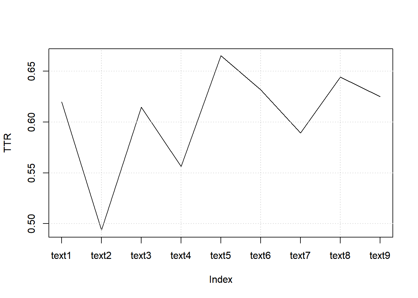
7.8.8.2.2 CTTR (Corrected Type-Token Ratio)
7.8.8.2.2.1 Computing CTTR
web_pages_txt_corpus_tok_no_punct_no_Stop_dfm_tstat_lexdiv_cttr <- textstat_lexdiv(web_pages_txt_corpus_tok_no_punct_no_Stop_dfm, measure = "CTTR")
head(web_pages_txt_corpus_tok_no_punct_no_Stop_dfm_tstat_lexdiv_cttr, 5)
## document CTTR
## 1 text1 8.009070
## 2 text2 7.599967
## 3 text3 7.701538
## 4 text4 9.809930
## 5 text5 6.8475657.8.8.2.2.2 Plotting TTR
plot(web_pages_txt_corpus_tok_no_punct_no_Stop_dfm_tstat_lexdiv_cttr$CTTR, type = "l", xaxt = "n", xlab = NULL, ylab = "CTTR")
grid()
axis(1, at = seq_len(nrow(web_pages_txt_corpus_tok_no_punct_no_Stop_dfm_tstat_lexdiv_cttr)), labels = web_pages_txt_corpus_tok_no_punct_no_Stop_dfm_tstat_lexdiv_cttr$document)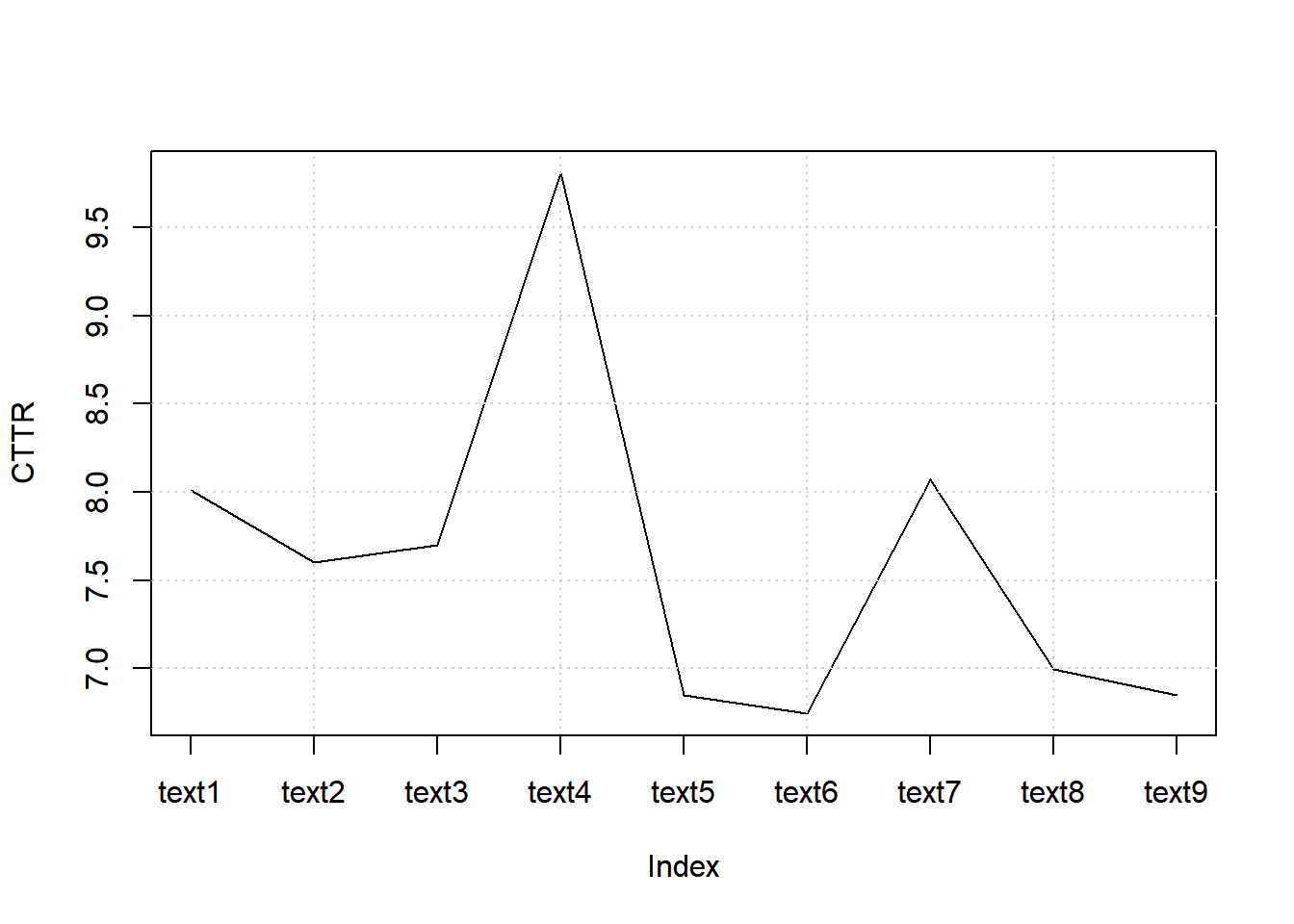
7.8.8.2.3 K (Yule’s K)
7.8.8.2.3.1 Computing K
web_pages_txt_corpus_tok_no_punct_no_Stop_dfm_tstat_lexdiv_K <- textstat_lexdiv(web_pages_txt_corpus_tok_no_punct_no_Stop_dfm, measure = "K")
head(web_pages_txt_corpus_tok_no_punct_no_Stop_dfm_tstat_lexdiv_K, 5)
## document K
## 1 text1 101.11513
## 2 text2 76.55468
## 3 text3 83.57337
## 4 text4 58.77731
## 5 text5 90.334647.8.8.2.3.2 Plotting K
plot(web_pages_txt_corpus_tok_no_punct_no_Stop_dfm_tstat_lexdiv_K$K, type = "l", xaxt = "n", xlab = NULL, ylab = expression(italic(K)))
grid()
axis(1, at = seq_len(nrow(web_pages_txt_corpus_tok_no_punct_no_Stop_dfm_tstat_lexdiv_K)), labels = web_pages_txt_corpus_tok_no_punct_no_Stop_dfm_tstat_lexdiv_K$document)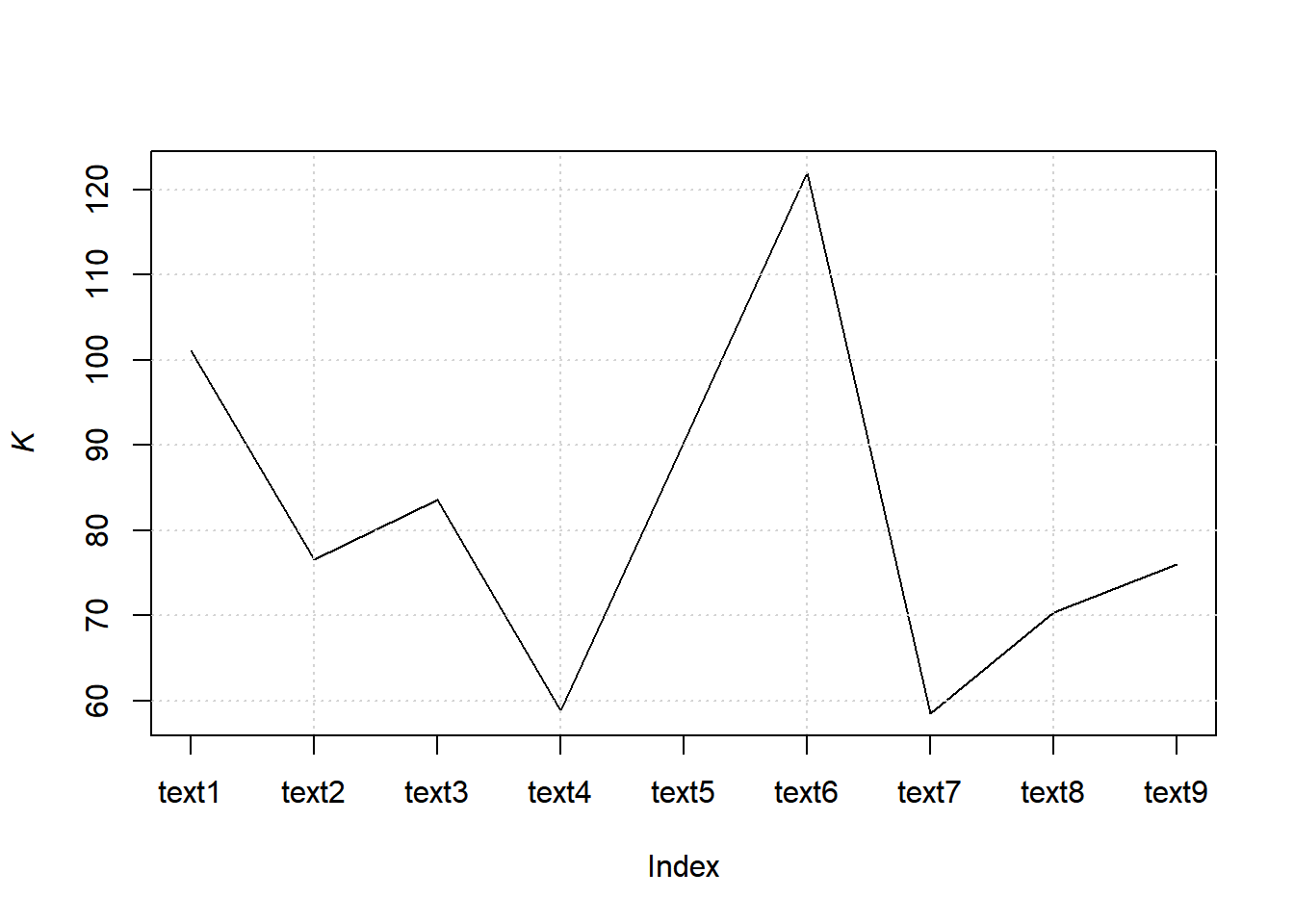
7.8.8.3 Keyness - relative frequency analysis
The relative frequency analysis allows to provide a statistical analysis of frequent words as a function of a target reference level. For this dataset, we do not have a specific target. Hence the comparison is done based on the full dataset.
7.8.8.3.1 Computing keyness
web_pages_txt_corpus_tok_no_punct_no_Stop_dfm_tstat_key <- textstat_keyness(web_pages_txt_corpus_tok_no_punct_no_Stop_dfm)
head(web_pages_txt_corpus_tok_no_punct_no_Stop_dfm_tstat_key, 10)
## feature chi2 p n_target n_reference
## 1 ggplot2 239.75832 0.000000e+00 26 2
## 2 faq 62.24016 2.997602e-15 7 0
## 3 graphics 62.24016 2.997602e-15 7 0
## 4 chang 20.95548 4.700802e-06 3 0
## 5 kara 20.95548 4.700802e-06 3 0
## 6 lin 20.95548 4.700802e-06 3 0
## 7 pedersen 20.95548 4.700802e-06 3 0
## 8 winston 20.95548 4.700802e-06 3 0
## 9 woo 20.95548 4.700802e-06 3 0
## 10 author 19.93531 8.010706e-06 10 20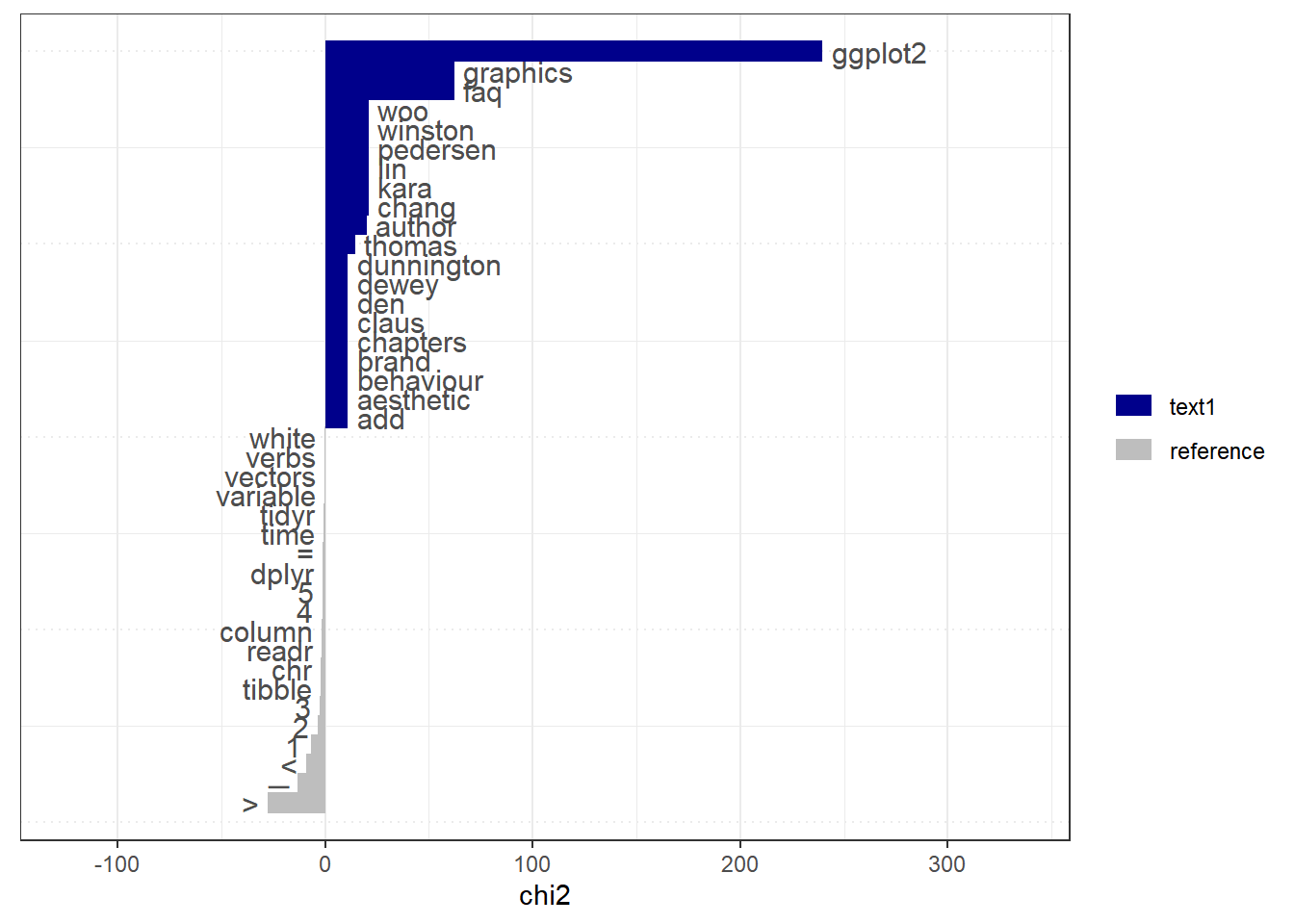
7.8.8.4 Collocations - scoring multi-word expressions
A collocation analysis is a way to identify contiguous collocations of words, i.e., multi-word expressions. Depending on the language, these can be identified based on capitalisation (e.g., proper names) as in English texts. However, this is not the same across languages.
We look for capital letters in our text. The result provides Wald’s Lamda and z statistics. Usually, any z value higher or equal to 2 is statistically significant. To compute p values, we use the probability of a normal distribution based on a mean of 0 and an SD of 1. This is appended to the table.
web_pages_txt_corpus_tok_no_punct_no_Stop_tstat_col_caps <- tokens_select(web_pages_txt_corpus_tok_no_punct_no_Stop, pattern = c("^[A-Z]", "^[a-z]"), valuetype = "regex", case_insensitive = FALSE, padding = TRUE) %>%  textstat_collocations(min_count = 10) %>% mutate(p_value = 1 - pnorm(z, 0, 1))
web_pages_txt_corpus_tok_no_punct_no_Stop_tstat_col_caps
## collocation count count_nested length lambda z p_value
## 1 pak pak 12 0 2 7.072542 11.355113 0.000000e+00
## 2 hadley wickham 18 0 2 12.595987 6.255673 1.979027e-10
## 3 code conduct 13 0 2 8.613831 5.908195 1.729383e-097.8.8.5 Word clouds
We can use word clouds of the top 100 words
set.seed(132)
web_pages_txt_corpus_tok_no_punct_no_Stop_dfm %>%
  textplot_wordcloud(max_words = 100, color = brewer.pal(8, "Dark2"))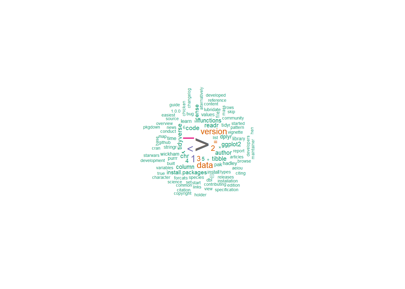
7.8.8.6 Network of feature co-occurrences
A Network of feature co-occurrences allows to obtain association plot of word usage. We use an fcm (feature co-occurrence matrix) based on our DFM.
set.seed(144)
web_pages_txt_corpus_tok_no_punct_no_Stop_dfm %>%
  dfm_trim(min_termfreq = 20) %>%
  textplot_network(min_freq = 0.5)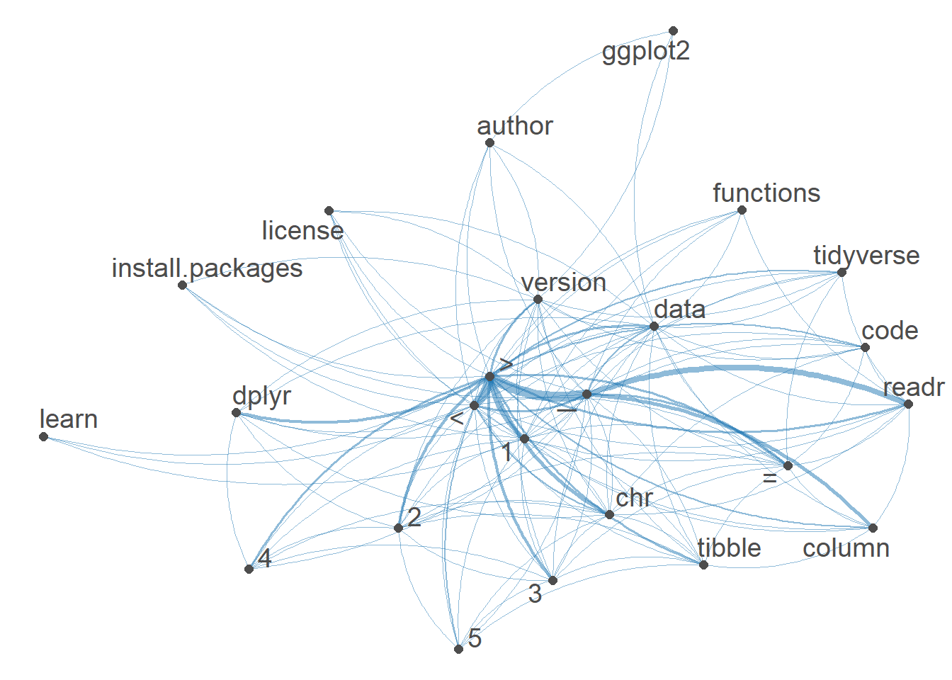
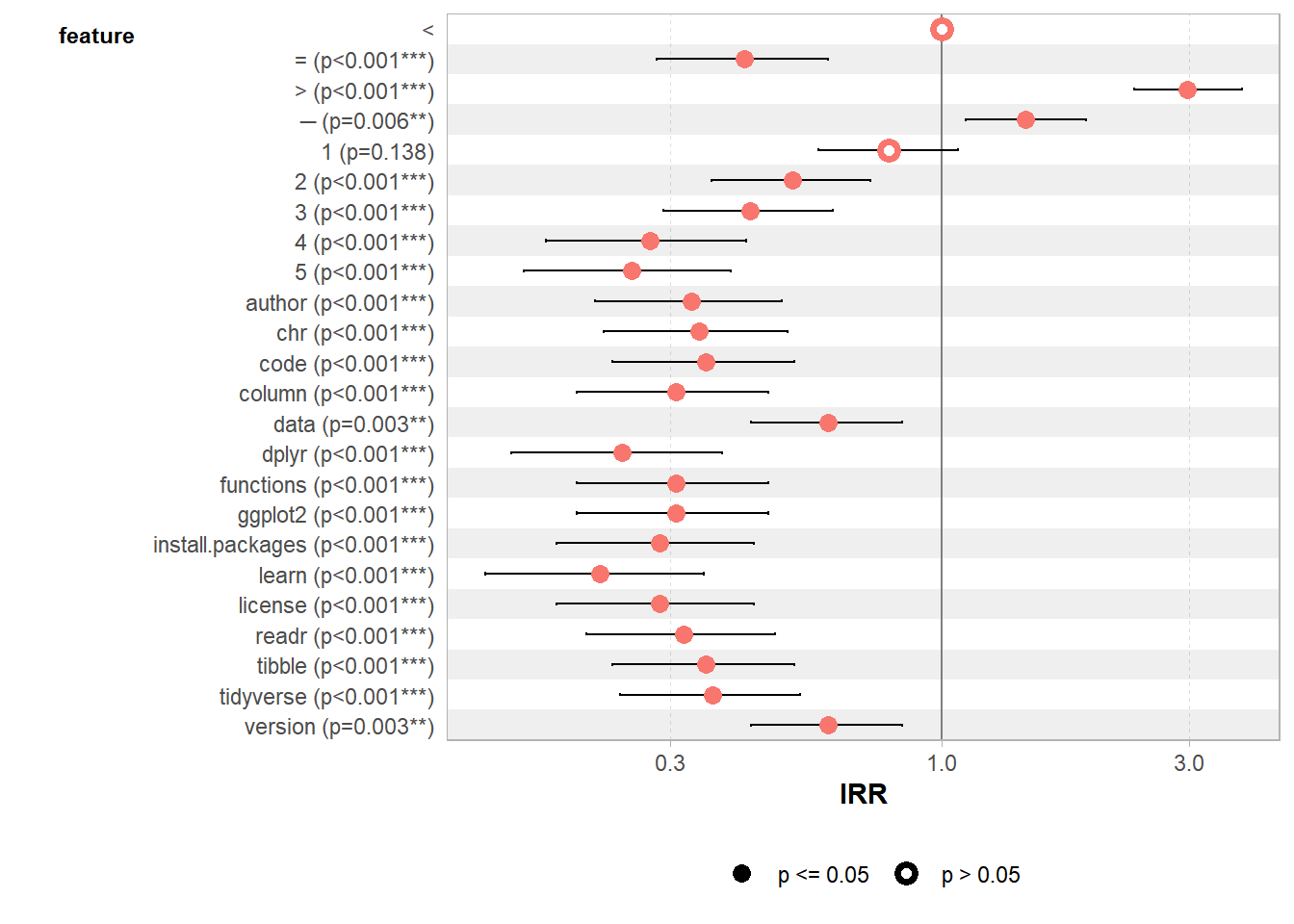
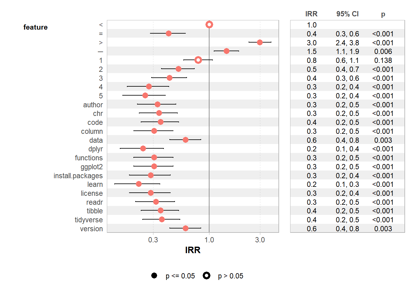
7.8.8.7 Poisson regression
Finally, we run a GLM with a poisson family to evaluate the significance level of our most frequent words.
7.8.8.7.1 Computing GLM
web_pages_txt_corpus_GLM <- web_pages_txt_corpus_tok_no_punct_no_Stop_dfm_freq %>%
  filter(frequency >= 20) %>%
  glm(frequency ~ feature, data = ., family = "poisson")
summary(web_pages_txt_corpus_GLM)
##
## Call:
## glm(formula = frequency ~ feature, family = "poisson", data = .)
##
## Coefficients:
## Estimate Std. Error z value Pr(>|z|)
## (Intercept) 4.5109 0.1048 43.031 < 2e-16 ***
## feature= -0.8733 0.1931 -4.521 6.14e-06 ***
## feature> 1.0913 0.1212 9.007 < 2e-16 ***
## feature─ 0.3719 0.1363 2.730 0.006337 **
## feature1 -0.2342 0.1577 -1.485 0.137597
## feature2 -0.6607 0.1796 -3.678 0.000235 ***
## feature3 -0.8473 0.1914 -4.427 9.55e-06 ***
## feature4 -1.2920 0.2258 -5.722 1.06e-08 ***
## feature5 -1.3754 0.2334 -5.893 3.79e-09 ***
## featureauthor -1.1097 0.2105 -5.271 1.36e-07 ***
## featurechr -1.0769 0.2080 -5.178 2.24e-07 ***
## featurecode -1.0451 0.2055 -5.085 3.67e-07 ***
## featurecolumn -1.1787 0.2161 -5.454 4.93e-08 ***
## featuredata -0.5035 0.1708 -2.948 0.003197 **
## featuredplyr -1.4198 0.2376 -5.976 2.28e-09 ***
## featurefunctions -1.1787 0.2161 -5.454 4.93e-08 ***
## featureggplot2 -1.1787 0.2161 -5.454 4.93e-08 ***
## featureinstall.packages -1.2528 0.2224 -5.634 1.77e-08 ***
## featurelearn -1.5151 0.2470 -6.135 8.51e-10 ***
## featurelicense -1.2528 0.2224 -5.634 1.77e-08 ***
## featurereadr -1.1436 0.2132 -5.363 8.20e-08 ***
## featuretibble -1.0451 0.2055 -5.085 3.67e-07 ***
## featuretidyverse -1.0144 0.2032 -4.992 5.98e-07 ***
## featureversion -0.5035 0.1708 -2.948 0.003197 **
## ---
## Signif. codes: 0 '***' 0.001 '**' 0.01 '*' 0.05 '.' 0.1 ' ' 1
##
## (Dispersion parameter for poisson family taken to be 1)
##
## Null deviance: 7.9759e+02 on 23 degrees of freedom
## Residual deviance: -1.6431e-14 on 0 degrees of freedom
## AIC: 180.25
##
## Number of Fisher Scoring iterations: 3