3.3 Correlation tests

3.3.1 Correlation does not imply causation!

There is a general misconception that when one conducts a correlation test (see below), we can explain causation. An excellent example is borrowed from wikipedia. It is not because two variables are correlated (positively or negatively) that one explains the reasons behind the second!

If you want to evaluate the cause of an effect then inferential statistics that we cover after the correlation tests are the ones to go for.

3.3.2 Basic correlations

Let us start with a basic correlation test. We want to evaluate if two numeric variables are correlated with each other.

We use the function cor to obtain the pearson correlation and cor.test to run a basic correlation test on our data with significance testing

cor(english$RTlexdec, english$RTnaming, method = "pearson")

## [1] 0.7587033

cor.test(english$RTlexdec, english$RTnaming)

## 
##  Pearson's product-moment correlation
## 
## data:  english$RTlexdec and english$RTnaming
## t = 78.699, df = 4566, p-value < 2.2e-16
## alternative hypothesis: true correlation is not equal to 0
## 95 percent confidence interval:
##  0.7461195 0.7707453
## sample estimates:
##       cor 
## 0.7587033

What these results are telling us? There is a positive correlation between RTlexdec and RTnaming. The correlation coefficient (R²) is 0.76 (limits between -1 and 1). This correlation is statistically significant with a t value of 78.699, degrees of freedom of 4566 and a p-value < 2.2e-16.

What are the degrees of freedom? These relate to number of total observations - number of comparisons. Here we have 4568 observations in the dataset, and two comparisons, hence 4568 - 2 = 4566.

For the p value, there is a threshold we usually use. This threshold is p = 0.05. This threshold means we have a minimum to consider any difference as significant or not. 0.05 means that we have a probability to find a significant difference that is at 5% or lower. IN our case, the p value is lower that 2.2e-16. How to interpret this number? this tells us to add 15 0s before the 2!! i.e., 0.0000000000000002. This probability is very (very!!) low. So we conclude that there is a statistically significant correlation between the two variables.

The formula to calculate the t value is below.

x̄ = sample mean μ0 = population mean s = sample standard deviation n = sample size

The p value is influenced by various factors, number of observations, strength of the difference, mean values, etc.. You should always be careful with interpreting p values taking everything else into account.

3.3.3 Using the package corrplot

Above, we did a correlation test on two predictors. What if we want to obtain a nice plot of all numeric predictors and add significance levels?

3.3.3.1 Correlation plots

corr <- 
  english %>% 
  select(where(is.numeric)) %>% 
  cor()
corrplot(corr, method = 'ellipse', type = 'upper')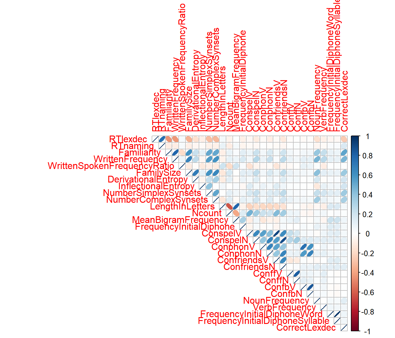

3.3.3.2 More advanced

Let’s first compute the correlations between all numeric variables and plot these with the p values

## correlation using "corrplot"
## based on the function `rcorr' from the `Hmisc` package
## Need to change dataframe into a matrix
corr <- 
  english %>% 
  select(where(is.numeric)) %>% 
  data.matrix(english) %>% 
  rcorr(type = "pearson")
# use corrplot to obtain a nice correlation plot!
corrplot(corr$r, p.mat = corr$P,
         addCoef.col = "black", diag = FALSE, type = "upper", tl.srt = 55)

english %>% 
  group_by(AgeSubject) %>% 
  summarise(mean = mean(RTlexdec),
            sd = sd(RTlexdec))

## # A tibble: 2 × 3
##   AgeSubject  mean    sd
##   <fct>      <dbl> <dbl>
## 1 old         6.66 0.116
## 2 young       6.44 0.106