9.5 Issues with GLM (and regression analyses in general)
9.5.1 Correlation tests
Below, we look at two predictors that are correlated with each other: Z3-Z2 (F3-F2 in Bark) and A2*-A3* (normalised amplitude differences between harmonics closest to F2 and F3). The results of the correlation test shows the two predictors to negatively correlate with each other at a rate of -0.87.
##
##  Pearson's product-moment correlation
##
## data:  dfPharV2$Z3mnZ2 and dfPharV2$A2mnA3
## t = -35.864, df = 400, p-value < 2.2e-16
## alternative hypothesis: true correlation is not equal to 0
## 95 percent confidence interval:
##  -0.8947506 -0.8480066
## sample estimates:
##        cor
## -0.8733751
9.5.2 Plots to visualise the data

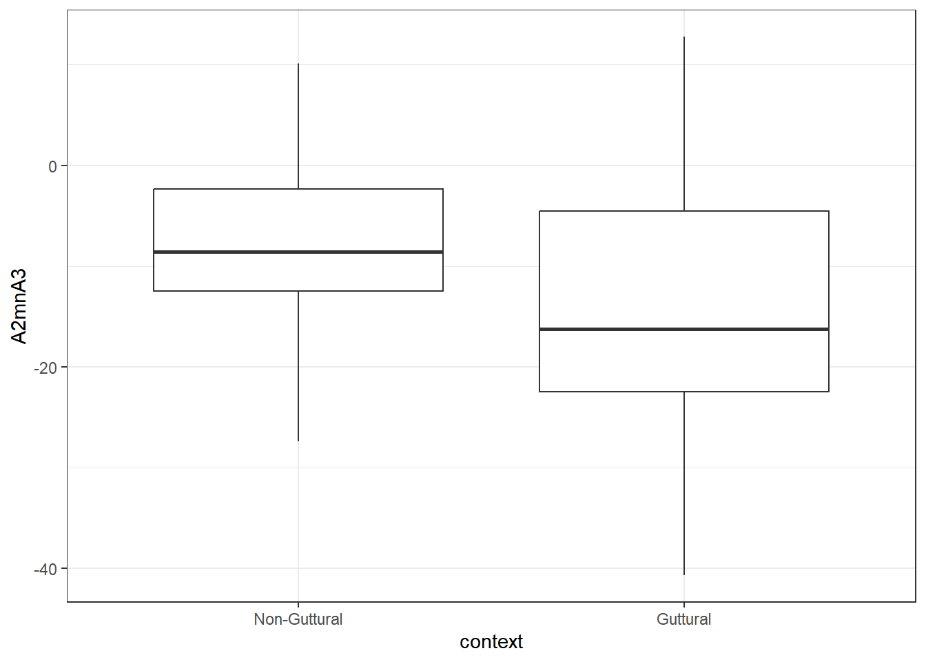
As we see from the plot, Z3-Z2 is higher in the guttural, whereas A2*-A3* is lower.
9.5.3 GLM on correlated data
9.5.3.1 Model specifications and issues
Let’s run a logistic regression as a classification tool to predict the context as a function of each predictor separately and then combined.
##
## Call:
## glm(formula = context ~ Z3mnZ2, family = binomial, data = .)
##
## Coefficients:
##             Estimate Std. Error z value Pr(>|z|)
## (Intercept) -0.99451    0.23061  -4.313 1.61e-05 ***
## Z3mnZ2       0.17440    0.04553   3.831 0.000128 ***
## ---
## Signif. codes:  0 '***' 0.001 '**' 0.01 '*' 0.05 '.' 0.1 ' ' 1
##
## (Dispersion parameter for binomial family taken to be 1)
##
##     Null deviance: 552.89  on 401  degrees of freedom
## Residual deviance: 537.74  on 400  degrees of freedom
## AIC: 541.74
##
## Number of Fisher Scoring iterations: 4##
## Call:
## glm(formula = context ~ A2mnA3, family = binomial, data = .)
##
## Coefficients:
## Estimate Std. Error z value Pr(>|z|)
## (Intercept) -0.98961 0.16632 -5.950 2.68e-09 ***
## A2mnA3 -0.06973 0.01122 -6.215 5.12e-10 ***
## ---
## Signif. codes: 0 '***' 0.001 '**' 0.01 '*' 0.05 '.' 0.1 ' ' 1
##
## (Dispersion parameter for binomial family taken to be 1)
##
## Null deviance: 552.89 on 401 degrees of freedom
## Residual deviance: 508.51 on 400 degrees of freedom
## AIC: 512.51
##
## Number of Fisher Scoring iterations: 4##
## Call:
## glm(formula = context ~ Z3mnZ2 + A2mnA3, family = binomial, data = .)
##
## Coefficients:
## Estimate Std. Error z value Pr(>|z|)
## (Intercept) -0.10996 0.27830 -0.395 0.692754
## Z3mnZ2 -0.39266 0.10201 -3.849 0.000118 ***
## A2mnA3 -0.14930 0.02418 -6.175 6.61e-10 ***
## ---
## Signif. codes: 0 '***' 0.001 '**' 0.01 '*' 0.05 '.' 0.1 ' ' 1
##
## (Dispersion parameter for binomial family taken to be 1)
##
## Null deviance: 552.89 on 401 degrees of freedom
## Residual deviance: 492.50 on 399 degrees of freedom
## AIC: 498.5
##
## Number of Fisher Scoring iterations: 4##
## Call:
## glm(formula = context ~ Z3mnZ2 * A2mnA3, family = binomial, data = .)
##
## Coefficients:
## Estimate Std. Error z value Pr(>|z|)
## (Intercept) 0.398028 0.337189 1.180 0.23783
## Z3mnZ2 -0.583131 0.131602 -4.431 9.38e-06 ***
## A2mnA3 -0.091045 0.031870 -2.857 0.00428 **
## Z3mnZ2:A2mnA3 -0.014581 0.005553 -2.626 0.00865 **
## ---
## Signif. codes: 0 '***' 0.001 '**' 0.01 '*' 0.05 '.' 0.1 ' ' 1
##
## (Dispersion parameter for binomial family taken to be 1)
##
## Null deviance: 552.89 on 401 degrees of freedom
## Residual deviance: 485.41 on 398 degrees of freedom
## AIC: 493.41
##
## Number of Fisher Scoring iterations: 4When looking at the three models above, it is clear that the log odd value for Z3-Z2 is positive, whereas it is negative for A2*-A3*. When adding the two predictors together, there is clear suppression: the coefficients for both predictors are now negative. The relatively high correlation between the predictors affected the coefficients and changed the direction of the slope; collinearity is harmful for any regression analysis. When we use an interaction term, the coefficients are all negative, leading to confusions in interpreting the results.
9.5.3.2 Checking collinearity
To check for collinearity, we can use the vif function from the car package. The vif stands for the “Variance Inflation Factor (VIF)”. This is a measure of how much the variance of a regression coefficient is increased due to collinearity. A VIF value below 5 indicates that there is low level of collinearity; between 5 and 10, that there a moderate level of collinearity and above 10 indicates potential collinearity issues.
9.5.3.2.1 Simple model
##   Z3mnZ2   A2mnA3
## 4.319093 4.319093
The values here are close to 5, which indicates a moderate level of collinearity. This is appropriate , but it is not ideal either.
9.5.3.2.2 Interaction model
## there are higher-order terms (interactions) in this model
## consider setting type = 'predictor'; see ?vif
## Z3mnZ2 A2mnA3 Z3mnZ2:A2mnA3
## 7.151205 7.551354 11.244070When using interaction, the vif values no increase to more than 5 for the individual predictors, and to 11 for the interaction
We use the function check_collinearity()
## Model has interaction terms. VIFs might be inflated.
##   Try to center the variables used for the interaction, or check
##   multicollinearity among predictors of a model without interaction terms.
## # Check for Multicollinearity
##
## Moderate Correlation
##
## Term VIF VIF 95% CI adj. VIF Tolerance Tolerance 95% CI
## Z3mnZ2 7.15 [6.00, 8.57] 2.67 0.14 [0.12, 0.17]
## A2mnA3 7.55 [6.33, 9.06] 2.75 0.13 [0.11, 0.16]
##
## High Correlation
##
## Term VIF VIF 95% CI adj. VIF Tolerance Tolerance 95% CI
## Z3mnZ2:A2mnA3 11.24 [9.37, 13.53] 3.35 0.09 [0.07, 0.11]dfPharV2 %>% glm(context ~ Z3mnZ2 * A2mnA3, data = ., family = binomial) %>%
check_collinearity() %>% plot()## Model has interaction terms. VIFs might be inflated.
## Try to center the variables used for the interaction, or check
## multicollinearity among predictors of a model without interaction terms.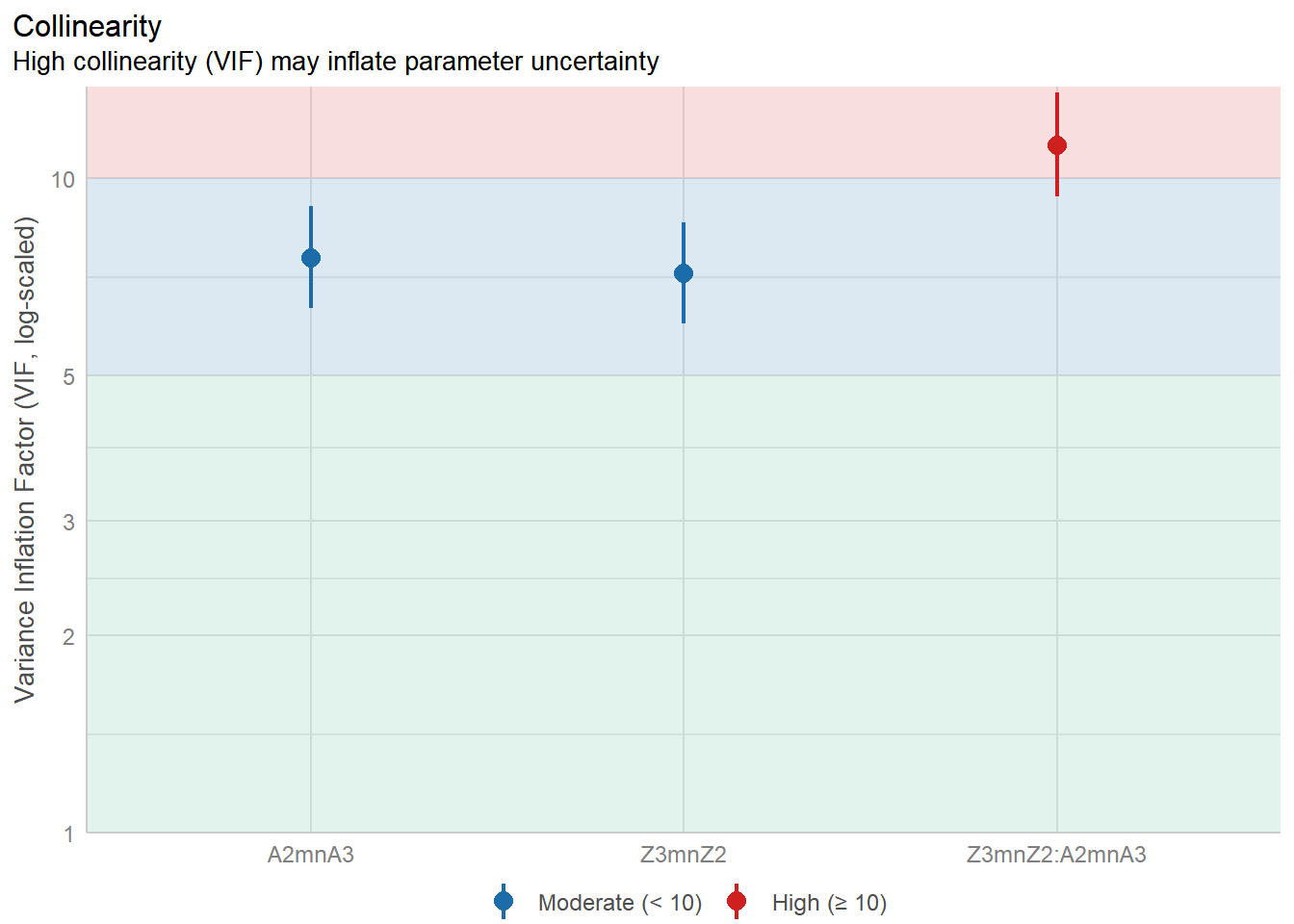
9.5.3.3 Full dataset
We run the logistic regression on the full dataset to evaluate the levels of collinearity
9.5.3.3.1 vif()
##           CPP        Energy         H1A1c         H1A2c         H1A3c
## -2.295300e+00 -1.985664e+00 -1.912497e+08 -5.449839e+08 -2.409111e+08
##         H1H2c         H2H4c       H2KH5Kc         H42Kc         HNR05
##  4.818970e-02 -4.030192e+00 -3.492308e+00  1.205078e+01 -4.429782e+01
##         HNR15         HNR25         HNR35           SHR           soe
##  5.987851e+00 -1.699119e+01 -1.828131e+01  9.651994e-01  3.750546e+00
##        Z1mnZ0        Z2mnZ1        Z3mnZ2        Z4mnZ3        F0Bark
##  1.160041e+01  7.672639e+01  1.574462e+01 -1.102098e+00  5.194514e+01
##        A1mnA2        A1mnA3        A2mnA3
## -3.515054e+14  2.292446e+15 -6.759060e+15
9.5.3.3.2 check_collinearity()
## The variance-covariance matrix is not positive definite. Returning the
##   nearest positive definite matrix now.
##   This ensures that eigenvalues are all positive real numbers, and
##   thereby, for instance, it is possible to calculate standard errors for
##   all relevant parameters.
## Warning in stats::qlogis(r): NaNs produced## # Check for Multicollinearity
##
## Low Correlation
##
## Term VIF VIF 95% CI adj. VIF Tolerance Tolerance 95% CI
## CPP 1.00 [ 1.00, Inf] 1.00 1.00 [0.00, 1.00]
## Energy 1.00 [ 1.00, Inf] 1.00 1.00 [0.00, 1.00]
## H1A1c 1.00 [ 1.00, Inf] 1.00 1.00 [0.00, 1.00]
## H1A2c 1.00 [ 1.00, Inf] 1.00 1.00 [0.00, 1.00]
## H1A3c 1.00 [ 1.00, Inf] 1.00 1.00 [0.00, 1.00]
## H1H2c 1.00 [ 1.00, Inf] 1.00 1.00 [0.00, 1.00]
## H2H4c 1.00 [ 1.00, Inf] 1.00 1.00 [0.00, 1.00]
## H2KH5Kc 1.00 [ 1.00, Inf] 1.00 1.00 [0.00, 1.00]
## H42Kc 1.00 [ 1.00, Inf] 1.00 1.00 [0.00, 1.00]
## HNR05 1.00 [ 1.00, Inf] 1.00 1.00 [0.00, 1.00]
## HNR15 1.00 [ 1.00, Inf] 1.00 1.00 [0.00, 1.00]
## HNR25 1.00 [ 1.00, Inf] 1.00 1.00 [0.00, 1.00]
## HNR35 1.00 [ 1.00, Inf] 1.00 1.00 [0.00, 1.00]
## SHR 1.00 [ 1.00, Inf] 1.00 1.00 [0.00, 1.00]
## soe 1.00 1.00 1.00
## Z1mnZ0 1.00 1.00 1.00
## Z2mnZ1 1.00 1.00 1.00
## Z3mnZ2 1.00 [ 1.00, Inf] 1.00 1.00 [0.00, 1.00]
## Z4mnZ3 1.00 1.00 1.00
## F0Bark 1.00 1.00 1.00
##
## High Correlation
##
## Term VIF VIF 95% CI adj. VIF Tolerance Tolerance 95% CI
## A1mnA2 2.22e+07 [1.85e+07, 2.67e+07] 4714.04 4.50e-08 [0.00, 0.00]
## A1mnA3 2.22e+07 [1.85e+07, 2.67e+07] 4714.04 4.50e-08 [0.00, 0.00]
## A2mnA3 2.22e+07 [1.85e+07, 2.67e+07] 4714.05 4.50e-08 [0.00, 0.00]## The variance-covariance matrix is not positive definite. Returning the
## nearest positive definite matrix now.
## This ensures that eigenvalues are all positive real numbers, and
## thereby, for instance, it is possible to calculate standard errors for
## all relevant parameters.## Warning in stats::qlogis(r): NaNs produced## Warning: Removed 5 rows containing missing values or values outside the scale
## range (`geom_segment()`).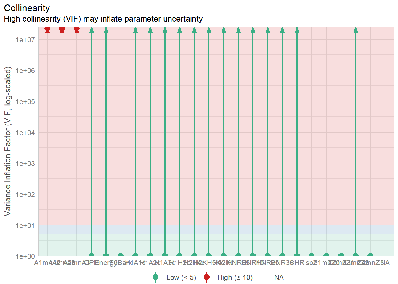
9.5.4 Conclusion
The more complex your regression model becomes, the higher level of collinearity one can see. This is a known issue in regression analyses, and without applying appropriate approaches, e.g., verifying the collinearity in the data; choosing non-correlated predictors, etc.., the models become inflated and the confidence in the results becomes reduced.
There are various solutions to this issue, such as removing collinear predictors, using PCA to obtain orthogonal dimension (i.e., non-correlated dimensions), etc.. Another solution is to use decision trees and Random Forest. Both are very well known to deal with collinearity and to make sense of multivariate predictors.