3.2 Inferential statistics
3.2.1 Introduction
What do we mean by inferential statistics?
We want to evaluate if there are differences observed between two groups of datapoints and if these differences are statistically significant.
For this, we need to pay attention to the format of our outcome and predictors. An outcome is the response variable (or dependent variable); a predictor is our independent variable(s). This is fed into our equation
\(y = x\beta + \varepsilon\)
where:
\(y\) \(\rightarrow\) outcome (DV) \(\Rightarrow\) known
\(x\) \(\rightarrow\) fixed effect (IV) \(\Rightarrow\) known
\(\beta\) \(\rightarrow\) coefficient of fixed effect \(\Rightarrow\) unknown
\(\varepsilon\) \(\rightarrow\) random error term \(\Rightarrow\) unknown
3.2.2 Hypothesis testing
In the approach that this book follows, we use a frequentist approach to hypothesis testing. By frequentist we mean when modelling the relationship between an outcome and a predictor, we are interested in testing if the predictor has a clear and statistically significant influence on the outcome. When evaluating this, we try to reject the null hypothesis (H\(_0\)) in favour of the alternative hypothesis (H\(_1\)).
The null hypothesis (H\(_0\)) is the hypothesis we make that there is no statistical evidence in favour of an effect nor of a difference between the groups. The alternative hypothesis (H\(_1\)) is the hypothesis we make to reject the null hypothesis and there is indeed a statistical evidence in favour of an effect or a difference between the groups.
3.2.3 Type of outcomes
It is important to know the class of the outcome before doing any pre-data analyses or inferential statistics. Outcome classes can be one of:
Numeric: As an example, we have length/width of leaf; height of mountain; fundamental frequency of the voice; etc. These are generally modelled with aGaussiandistribution These aretruenumbers and we can use summaries, t-tests, linear models, etc. Integers are a family of numeric variables and can still be considered as a normal numeric variable. Count data are numbers related to a category. In general, these are related to the second type of outcomes, and should be analysed using a poisson logistic regressionCategorical(Unordered): Observations for two or more categories. As an example, we can have gender of a speaker (male or female); responses to a True vs False perception tests; Colour (unordered) categorisation, e.g., red, blue, yellow, orange, etc.. For these we can use a Generalised Linear Model (binomial or multinomial) or a simple chi-square test.Categorical(Ordered): When you run a rating experiment, where the outcome is eithernumeric(i.e., 1, 2, 3, 4, 5) orcategories(i.e., disagree, neutral, agree). Thenumericoption is NOT a true number as for the participant, these are categories. Cumulative Logit models (or Generalised Linear Model with a cumulative function) are used. The mean is meaningless here, and the median is a preferred descriptive statistic.
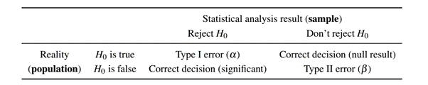
3.2.4 Types of Errors?
In the literature, we discuss various types of errors in statistical models. There are four different types, and the excellent Sonderegger (2023) book (Sonderegger, M. (2023). Regression Modeling for Linguistic Data. The MIT Press.) summarises these nicely. Here are the four types:
Type I (or “false positive” or error \(\alpha\)) \(\Rightarrow\) falsely concluding there is an effect when none exists. (generally due to inaccurate modelling strategies)
Type II (or “false negative” or error \(\beta\))) \(\Rightarrow\) falsely concluding there is no effect when one in fact exists (generally due to inaccurate modelling strategies)
Type S \(\Rightarrow\) Inaccurate sign (generally due to hidden multicollinearity and low power = 1- \(\beta\))
Type M \(\Rightarrow\) Inaccurate magnitude (generally due to hidden multicollinearity and low power = 1- \(\beta\))
It is important to note that the Type I and Type II errors are the most commonly discussed in the literature and are related to each other. Modelling is an art, and depending on model specifications, we can easily increase Type I and/or Type II errors. Type I is usually increased in the case of using inaccuratley specified model, e.g., not using a random effects structure when the data comes from multiple speakers and/or multiple items. Type II error is usually increased when there is an over specification of the model and/or not accounting for dependencies in the data. Type S and Type M are generally caused due to collinearity in the data, which causes instability in the model and leads to cases of suppression; a point discussed in chapter 9.