4.2 Random effects?
Random effects are used to account for the inter-dependencies in a dataset. In various domains, including linguistics, we often collect data from multiple Subjects, items, and utterances.
- Multiple Subjects
- Multiple Items (words)
- Multiple utterances where words are embedded
- Multiple listeners in perception experiments
In the last case, when designing our perception experiment, we can sometimes use multiple items, coming from multiple utterances and from multiple subjects!
When the data comes from multiple subjects, items, etc.., there is a clear inter-dependency in the data. Without appropriately accounting for these, inter-dependencies, we are at a greater risk of increasing Type I Error and in some cases Type 2 error (see chapter 3 on the various types of errors).
This is the equation that represents the error term associated with random effects:
\(y = x\beta + \varepsilon + Zu\)
where:
- \(y\) \(\rightarrow\) outcome (DV) \(\Rightarrow\) known
- \(x\) \(\rightarrow\) fixed effect (IV) \(\Rightarrow\) known
- \(\beta\) \(\rightarrow\) coefficient of fixed effect \(\Rightarrow\) unknown
- \(\varepsilon\) \(\rightarrow\) random error term \(\Rightarrow\) unknown
- \(Z\) \(\rightarrow\) random effects term \(\Rightarrow\) known
- \(u\) \(\rightarrow\) random effects coefficients \(\Rightarrow\) unknown
In a linear regression model (see chapter 3), the error term \(\varepsilon\) is a general error term related to the unexplained variance in the data. We see that this error term inscreases when we have inter-dependencies in the data unaccounted for (i.e., an increase in the \(\varepsilon\) leads to an increase in Type I error). In a random effects structure, some of this error is related to the \(Z\) and \(u\). These two will lead to a decrease in the error term \(\varepsilon\) meaning that we allowed the model to account for the inter-dependencies in the data. However, in some instances, the unexplained variance in the data can decrease drastically with the error term associated with random effects increasing drastically. In these cases, there is a clear increase in Type II error.
4.2.1 How to choose fixed and random effects
4.2.1.1 Fixed effects
Fixed effects are those that are part of the experimental conditions. If you have exhausted all levels of an experimental condition, then this goes into fixed effects.
Covariates are a special case. Covariates are independent variables that co-vary with the population. For instance, a speaker can either be a male or a female (from a physiological sex perspective not accounting for sociolinguistic gender). This physiological gender then covaries with our subjects, and in some instances, can be used to allow for the coefficients to be adjusted to account for this type ode dependency (or covariation).
4.2.1.2 Random effects
Random effects are random selections of the population you have and you want to generalise over them.
E.g., Speakers, listeners, items, utterances, corpora…. are all random effects because you are not using all the population of speakers, listeners, items, utterances or corpora in your data!
BUT.. Can Speakers, listeners, items, or utterances be included as fixed effects? Yes!! When you do this, it means you are interested in this specific population and want to evaluate differences specific to the population!!
4.2.2 What about Random Intercepts and Random Slopes
We often find references in the literature to specific notions of random intercepts and random slopes. To demonstrate what these mean (beyond the definitions), we look at an example. For example, using a simulated dataset (for more details see below under Linear Mixed-effects Models), figure A shows the predicted average Looking time. In the incongruent condition, there is a clear increase in the Looking time.
4.2.2.1 Random Intercepts
Random Intercepts are used to obtain averages of your population and these are used in your statistical model to estimate group-specific variations. These are represented in figure B. As can be seen here, the overall increase in looking time in the incongruent condition is confirmed and all subjects show this type of increase. However, what is important to note is that the intercepts (starting and ending times) per subject are different, but all subjects have the same slope. This is normal given that we did not allow subjects to covary with respect to the congruence-incongruence condition.
4.2.2.2 Random Intercepts and Random Slopes
When using Random Intercepts and Random Slopes, we mean that we allowed for averages per subject to be computed, in addition to allowing each subject’s variability with regards to the fixed effect to covary. The figure C shows this clearly. Not only that subjects have different intercepts (starting and ending times); they also have different slopes with some showing steeper slopes and others shallower slopes.
Random slopes are adjustments to the subjects’ observations as a function of the variable(s) of interest. Usually, any within-subject (or within-item) variable(s) is(are) to be included as a random slope(s), but you need to use model comparison to evaluate the need to use it.
plot_model(xmdl.Optimal, type = "pred", terms = "Cond", ci.lvl = 0.95, dodge = 0,
           show.legend = FALSE, title = "A. Predicted average LookingTime") + theme_bw() +
  geom_line() + coord_cartesian(ylim = c(-275, 2000)) +
plot_model(xmdl.rand.Interc, type = "pred", terms = c("Cond", "Subj"), pred.type = "re",
           ci.lvl = NA, dodge = 0, colors = paletteer_c("grDevices::rainbow",
                                                        length(unique(dataCong$Subj))),
           show.legend = FALSE, title = "B. Subject Intercepts of LookingTime") + theme_bw() +
  geom_line() + coord_cartesian(ylim = c(-275, 2000)) +
plot_model(xmdl.Optimal, type = "pred", terms = c("Cond", "Subj"), pred.type = "re",
           ci.lvl = NA, dodge = 0, colors = paletteer_c("grDevices::rainbow",
                                                        length(unique(dataCong$Subj))),
           show.legend = FALSE, title = "C. Subject Slopes of LookingTime") + theme_bw() +
  geom_line() + coord_cartesian(ylim = c(-275, 2000))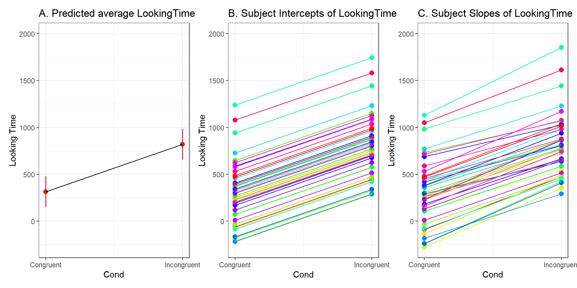
In the next section, we start by demonstrating the use of Linear Mixed-effects Models.