4.5 Cumulative Logit Link Mixed-effects Models
These models work perfectly with rating data. Ratings are inherently ordered, 1, 2, … n, and expect to observe an increase (or decrease) in overall ratings from 1 to n. To demonstrate this, we will use an example using the package “ordinal”.
We use two datasets. We previously ran these two models, however, in this subset of the full dataset, we did not take into account the fact that there were multiple producing speakers and items.
4.5.1 Ratings of percept of nasality
The first comes from a likert-scale a rating experiment where six participants rated the percept of nasality in the production of particular consonants in Arabic. The data came from nine producing subjects. The ratings were from 1 to 5, with 1 reflecting an oral percept; 5 a nasal percept.
4.5.1.1 Importing and pre-processing
We start by importing the data and process it. We change the reference level in the predictor
## # A tibble: 405 × 5
##    Response Context   Subject Item    Rater
##       <dbl> <chr>     <chr>   <chr>   <chr>
##  1        2 n-3       p04     noo3-w  R01
##  2        4 isolation p04     noo3-v  R01
##  3        2 o-3       p04     djuu3-w R01
##  4        4 isolation p04     djuu3-v R01
##  5        3 n-7       p04     nuu7-w  R01
##  6        3 isolation p04     nuu7-v  R01
##  7        1 3--3      p04     3oo3-w  R01
##  8        2 isolation p04     3oo3-v  R01
##  9        2 o-7       p04     loo7-w  R01
## 10        1 o-3       p04     bii3-w  R01
## # ℹ 395 more rows
rating <- rating %>%
mutate(Response = factor(Response),
Context = factor(Context),
Subject = factor(Subject),
Item = factor(Item)) %>%
mutate(Context = relevel(Context, "isolation"))
rating %>%
head(10)## # A tibble: 10 × 5
## Response Context Subject Item Rater
## <fct> <fct> <fct> <fct> <chr>
## 1 2 n-3 p04 noo3-w R01
## 2 4 isolation p04 noo3-v R01
## 3 2 o-3 p04 djuu3-w R01
## 4 4 isolation p04 djuu3-v R01
## 5 3 n-7 p04 nuu7-w R01
## 6 3 isolation p04 nuu7-v R01
## 7 1 3--3 p04 3oo3-w R01
## 8 2 isolation p04 3oo3-v R01
## 9 2 o-7 p04 loo7-w R01
## 10 1 o-3 p04 bii3-w R014.5.1.2 Model specifications
4.5.1.2.1 No random effects
We run our first clm model as a simple, i.e., with no random effects
##    user  system elapsed
## 0.02 0.00 0.01## formula: Response ~ Context
## data: .
##
## link threshold nobs logLik AIC niter max.grad cond.H
## logit flexible 405 -526.16 1086.31 5(0) 3.61e-09 1.3e+02
##
## Coefficients:
## Estimate Std. Error z value Pr(>|z|)
## Context3--3 -0.1384 0.5848 -0.237 0.8130
## Context3-n 3.5876 0.4721 7.600 2.96e-14 ***
## Context3-o -0.4977 0.3859 -1.290 0.1971
## Context7-n 2.3271 0.5079 4.582 4.60e-06 ***
## Context7-o 0.2904 0.4002 0.726 0.4680
## Contextn-3 2.8957 0.6685 4.331 1.48e-05 ***
## Contextn-7 2.2678 0.4978 4.556 5.22e-06 ***
## Contextn-n 2.8697 0.4317 6.647 2.99e-11 ***
## Contextn-o 3.5152 0.4397 7.994 1.30e-15 ***
## Contexto-3 -0.2540 0.4017 -0.632 0.5272
## Contexto-7 -0.6978 0.3769 -1.851 0.0641 .
## Contexto-n 2.9640 0.4159 7.126 1.03e-12 ***
## Contexto-o -0.6147 0.3934 -1.562 0.1182
## ---
## Signif. codes: 0 '***' 0.001 '**' 0.01 '*' 0.05 '.' 0.1 ' ' 1
##
## Threshold coefficients:
## Estimate Std. Error z value
## 1|2 -1.4615 0.2065 -7.077
## 2|3 0.4843 0.1824 2.655
## 3|4 1.5492 0.2044 7.578
## 4|5 3.1817 0.2632 12.0894.5.1.2.2 Random effects 1 - Intercepts only
We run our first clmm model as a simple, i.e., with random intercepts
##    user  system elapsed
## 4.70 0.20 4.96## Cumulative Link Mixed Model fitted with the Laplace approximation
##
## formula: Response ~ Context + (1 | Subject) + (1 | Item)
## data: .
##
## link threshold nobs logLik AIC niter max.grad cond.H
## logit flexible 405 -520.89 1079.79 1395(2832) 7.26e-04 1.2e+02
##
## Random effects:
## Groups Name Variance Std.Dev.
## Item (Intercept) 1.272e-14 1.128e-07
## Subject (Intercept) 1.942e-01 4.407e-01
## Number of groups: Item 45, Subject 9
##
## Coefficients:
## Estimate Std. Error z value Pr(>|z|)
## Context3--3 -0.1634 0.5798 -0.282 0.7781
## Context3-n 3.6779 0.4804 7.657 1.91e-14 ***
## Context3-o -0.5156 0.3873 -1.331 0.1831
## Context7-n 2.3775 0.5185 4.585 4.54e-06 ***
## Context7-o 0.3279 0.4046 0.810 0.4177
## Contextn-3 3.0361 0.6677 4.547 5.43e-06 ***
## Contextn-7 2.3599 0.4925 4.792 1.65e-06 ***
## Contextn-n 2.9633 0.4339 6.830 8.52e-12 ***
## Contextn-o 3.6644 0.4495 8.153 3.56e-16 ***
## Contexto-3 -0.2772 0.4000 -0.693 0.4883
## Contexto-7 -0.7334 0.3800 -1.930 0.0536 .
## Contexto-n 3.0672 0.4220 7.268 3.65e-13 ***
## Contexto-o -0.6505 0.4015 -1.620 0.1052
## ---
## Signif. codes: 0 '***' 0.001 '**' 0.01 '*' 0.05 '.' 0.1 ' ' 1
##
## Threshold coefficients:
## Estimate Std. Error z value
## 1|2 -1.5141 0.2554 -5.928
## 2|3 0.5077 0.2358 2.153
## 3|4 1.6039 0.2538 6.319
## 4|5 3.2921 0.3072 10.7184.5.1.2.3 Random effects 2 - Intercepts and Slopes
We run our second clmm model as a simple, i.e., with random intercepts and random slopes. Because the model will run for a while, we added an if condition to say f the model was run previously, simply load the rds file rather than running it.
system.time(mdl.clmm.Slope <- rating %>%
                                       clmm(Response ~ Context + (Context|Subject) + (1|Item), data = .))
## user system elapsed
## 939.72 48.50 1006.06## Cumulative Link Mixed Model fitted with the Laplace approximation
##
## formula: Response ~ Context + (Context | Subject) + (1 | Item)
## data: .
##
## link threshold nobs logLik AIC niter max.grad cond.H
## logit flexible 405 -492.53 1231.05 55305(218422) 8.87e-02 1.5e+04
##
## Random effects:
## Groups Name Variance Std.Dev. Corr
## Item (Intercept) 0.05939 0.2437
## Subject (Intercept) 0.70845 0.8417
## Context3--3 2.34447 1.5312 -0.755
## Context3-n 4.43319 2.1055 -0.258 0.654
## Context3-o 1.37733 1.1736 -0.677 0.985 0.649
## Context7-n 4.33218 2.0814 -0.544 0.729 0.389 0.709
## Context7-o 1.55843 1.2484 -0.809 0.740 0.068 0.682 0.431
## Contextn-3 7.99273 2.8271 -0.251 0.725 0.807 0.773 0.204
## Contextn-7 4.87737 2.2085 -0.276 0.563 0.516 0.553 -0.090
## Contextn-n 3.60679 1.8992 -0.659 0.924 0.662 0.916 0.420
## Contextn-o 2.26056 1.5035 -0.730 0.633 0.022 0.615 0.141
## Contexto-3 1.00547 1.0027 -0.159 0.484 0.443 0.513 -0.189
## Contexto-7 1.48508 1.2186 -0.889 0.738 0.196 0.637 0.456
## Contexto-n 2.76687 1.6634 -0.874 0.871 0.398 0.787 0.578
## Contexto-o 1.78059 1.3344 -0.883 0.645 0.300 0.547 0.739
##
##
##
##
##
##
##
##
## 0.336
## 0.547 0.824
## 0.744 0.867 0.825
## 0.915 0.429 0.639 0.747
## 0.457 0.840 0.969 0.771 0.626
## 0.946 0.290 0.511 0.721 0.811 0.359
## 0.919 0.469 0.581 0.837 0.769 0.434 0.970
## 0.561 0.031 -0.057 0.411 0.345 -0.221 0.723 0.733
## Number of groups: Item 45, Subject 9
##
## Coefficients:
## Estimate Std. Error z value Pr(>|z|)
## Context3--3 -0.2625 0.8280 -0.317 0.75120
## Context3-n 4.6025 0.9754 4.718 2.38e-06 ***
## Context3-o -0.5739 0.5821 -0.986 0.32413
## Context7-n 2.5260 0.9164 2.756 0.00584 **
## Context7-o 0.3748 0.6183 0.606 0.54433
## Contextn-3 4.1834 1.4119 2.963 0.00305 **
## Contextn-7 2.9393 0.9457 3.108 0.00188 **
## Contextn-n 3.5724 0.8166 4.375 1.21e-05 ***
## Contextn-o 4.4321 0.7515 5.898 3.69e-09 ***
## Contexto-3 -0.3567 0.5562 -0.641 0.52138
## Contexto-7 -0.8254 0.5861 -1.408 0.15905
## Contexto-n 3.6329 0.7410 4.903 9.44e-07 ***
## Contexto-o -0.6508 0.6248 -1.042 0.29755
## ---
## Signif. codes: 0 '***' 0.001 '**' 0.01 '*' 0.05 '.' 0.1 ' ' 1
##
## Threshold coefficients:
## Estimate Std. Error z value
## 1|2 -1.7147 0.3662 -4.682
## 2|3 0.5701 0.3481 1.638
## 3|4 1.8427 0.3666 5.026
## 4|5 3.9828 0.4399 9.0544.5.1.3 Testing significance
We can evaluate whether “Context” improves the model fit, by comparing a null model with our model. Of course “Context” is improving the model fit.
4.5.1.3.1 Null vs no random
## Likelihood ratio tests of cumulative link models:
##
##              formula:           link: threshold:
## mdl.clm.Null Response ~ 1       logit flexible
## mdl.clm      Response ~ Context logit flexible
##
##              no.par    AIC  logLik LR.stat df Pr(>Chisq)
## mdl.clm.Null      4 1281.1 -636.56
## mdl.clm          17 1086.3 -526.16   220.8 13  < 2.2e-16 ***
## ---
## Signif. codes:  0 '***' 0.001 '**' 0.01 '*' 0.05 '.' 0.1 ' ' 1
4.5.1.3.2 No random vs Random Intercepts
## Likelihood ratio tests of cumulative link models:
##
##              formula:                                        link: threshold:
## mdl.clm      Response ~ Context                              logit flexible
## mdl.clmm.Int Response ~ Context + (1 | Subject) + (1 | Item) logit flexible
##
##              no.par    AIC  logLik LR.stat df Pr(>Chisq)
## mdl.clm          17 1086.3 -526.16
## mdl.clmm.Int     19 1079.8 -520.89  10.525  2   0.005182 **
## ---
## Signif. codes:  0 '***' 0.001 '**' 0.01 '*' 0.05 '.' 0.1 ' ' 1
4.5.1.3.3 No random vs Random Intercepts
## Likelihood ratio tests of cumulative link models:
##
##                formula:                                              link:
## mdl.clmm.Int   Response ~ Context + (1 | Subject) + (1 | Item)       logit
## mdl.clmm.Slope Response ~ Context + (Context | Subject) + (1 | Item) logit
##                threshold:
## mdl.clmm.Int   flexible
## mdl.clmm.Slope flexible
##
##                no.par    AIC  logLik LR.stat  df Pr(>Chisq)
## mdl.clmm.Int       19 1079.8 -520.89
## mdl.clmm.Slope    123 1231.1 -492.53  56.737 104          1
The model comparison above shows that using random intercepts is enough in our case. By subject Random Slopes are not needed; subjects “seem” to show similarities in how they produced the items. In our publication, by Rater Random Slopes for context were needed.
4.5.1.4 Model’s fit
print(tab_model(mdl.clmm.Int, file = paste0("outputs/mdl.clmm.Int.html")))
htmltools::includeHTML("outputs/mdl.clmm.Int.html")| Response | |||
|---|---|---|---|
| Predictors | Odds Ratios | CI | p |
| 1|2 | 0.22 | 0.13 – 0.36 | <0.001 |
| 2|3 | 1.66 | 1.05 – 2.64 | 0.031 |
| 3|4 | 4.97 | 3.02 – 8.18 | <0.001 |
| 4|5 | 26.90 | 14.73 – 49.11 | <0.001 |
| Context3--3 | 0.85 | 0.27 – 2.65 | 0.778 |
| Context [3-n] | 39.56 | 15.43 – 101.43 | <0.001 |
| Context [3-o] | 0.60 | 0.28 – 1.28 | 0.183 |
| Context [7-n] | 10.78 | 3.90 – 29.78 | <0.001 |
| Context [7-o] | 1.39 | 0.63 – 3.07 | 0.418 |
| Contextn-3 | 20.82 | 5.63 – 77.07 | <0.001 |
| Contextn-7 | 10.59 | 4.03 – 27.80 | <0.001 |
| Context [n-n] | 19.36 | 8.27 – 45.32 | <0.001 |
| Context [n-o] | 39.03 | 16.17 – 94.19 | <0.001 |
| Contexto-3 | 0.76 | 0.35 – 1.66 | 0.488 |
| Contexto-7 | 0.48 | 0.23 – 1.01 | 0.054 |
| Context [o-n] | 21.48 | 9.39 – 49.12 | <0.001 |
| Context [o-o] | 0.52 | 0.24 – 1.15 | 0.105 |
| Random Effects | |||
| σ2 | 3.29 | ||
| τ00 Item | 0.00 | ||
| τ00 Subject | 0.19 | ||
| N Subject | 9 | ||
| N Item | 45 | ||
| Observations | 405 | ||
| Marginal R2 / Conditional R2 | 0.453 / NA | ||
4.5.1.5 Interpreting a cumulative model
As a way to interpret the model, we can look at the coefficients and make sense of the results. A CLM model is a Logistic model with a cumulative effect. The “Coefficients” are the estimates for each level of the fixed effect; the “Threshold coefficients” are those of the response. For the former, a negative coefficient indicates a negative association with the response; and a positive is positively associated with the response. The p values are indicating the significance of each level. For the “Threshold coefficients”, we can see the cumulative effects of ratings 1|2, 2|3, 3|4 and 4|5 which indicate an overall increase in the ratings from 1 to 5.
4.5.1.6 Plotting
4.5.1.6.1 No confidence intervals
We use a modified version of a plotting function that allows us to visualise the effects. For this, we use the base R plotting functions. The version below is without confidence intervals.
par(oma=c(1, 0, 0, 3),mgp=c(2, 1, 0))
xlimNas = c(min(mdl.clmm.Int$beta), max(mdl.clmm.Int$beta))
ylimNas = c(0,1)
plot(0,0,xlim=xlimNas, ylim=ylimNas, type="n", ylab=expression(Probability), xlab="", xaxt = "n",main="Predicted curves - Nasalisation",cex=2,cex.lab=1.5,cex.main=1.5,cex.axis=1.5)
axis(side = 1, at = c(0,mdl.clmm.Int$beta),labels = levels(rating$Context), las=2,cex=2,cex.lab=1.5,cex.axis=1.5)
xsNas = seq(xlimNas[1], xlimNas[2], length.out=100)
lines(xsNas, plogis(mdl.clmm.Int$Theta[1] - xsNas), col='black')
lines(xsNas, plogis(mdl.clmm.Int$Theta[2] - xsNas)-plogis(mdl.clmm.Int$Theta[1] - xsNas), col='red')
lines(xsNas, plogis(mdl.clmm.Int$Theta[3] - xsNas)-plogis(mdl.clmm.Int$Theta[2] - xsNas), col='green')
lines(xsNas, plogis(mdl.clmm.Int$Theta[4] - xsNas)-plogis(mdl.clmm.Int$Theta[3] - xsNas), col='orange')
lines(xsNas, 1-(plogis(mdl.clmm.Int$Theta[4] - xsNas)), col='blue')
abline(v=c(0,mdl.clmm.Int$beta),lty=3)
abline(h=0, lty="dashed")
abline(h=0.2, lty="dashed")
abline(h=0.4, lty="dashed")
abline(h=0.6, lty="dashed")
abline(h=0.8, lty="dashed")
abline(h=1, lty="dashed")

legend(par('usr')[2], par('usr')[4], bty='n', xpd=NA,lty=1, col=c("black", "red", "green", "orange", "blue"),
       legend=c("Oral", "2", "3", "4", "Nasal"),cex=0.75)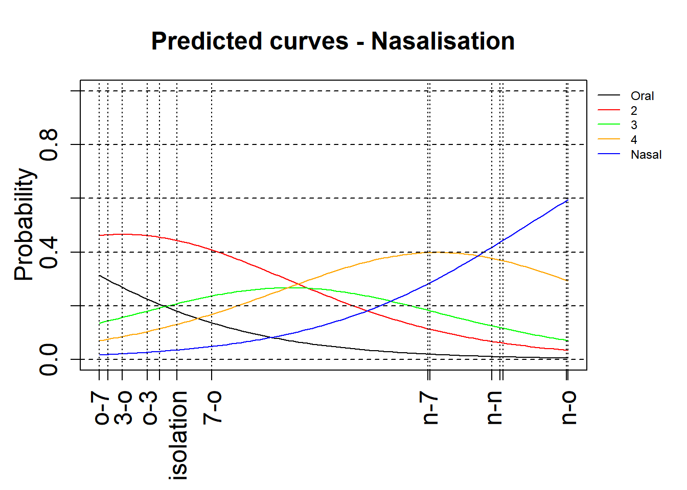
4.5.1.6.2 With confidence intervals
Here is an attempt to add the 97.5% confidence intervals to these plots. This is an experimental attempt and any feedback is welcome!
par(oma=c(1, 0, 0, 3),mgp=c(2, 1, 0))
xlimNas = c(min(mdl.clmm.Int$beta), max(mdl.clmm.Int$beta))
ylimNas = c(0,1)
plot(0,0,xlim=xlimNas, ylim=ylimNas, type="n", ylab=expression(Probability), xlab="", xaxt = "n",main="Predicted curves - Nasalisation",cex=2,cex.lab=1.5,cex.main=1.5,cex.axis=1.5)
axis(side = 1, at = c(0,mdl.clmm.Int$beta),labels = levels(rating$Context), las=2,cex=2,cex.lab=1.5,cex.axis=1.5)
xsNas = seq(xlimNas[1], xlimNas[2], length.out=100)


#+CI
lines(xsNas, plogis(mdl.clmm.Int$Theta[1]+(summary(mdl.clmm.Int)$coefficient[,2][[1]]/1.96) - xsNas), col='black')
lines(xsNas, plogis(mdl.clmm.Int$Theta[2]+(summary(mdl.clmm.Int)$coefficient[,2][[2]]/1.96) - xsNas)-plogis(mdl.clmm.Int$Theta[1]+(summary(mdl.clmm.Int)$coefficient[,2][[1]]/1.96) - xsNas), col='red')
lines(xsNas, plogis(mdl.clmm.Int$Theta[3]+(summary(mdl.clmm.Int)$coefficient[,2][[3]]/1.96) - xsNas)-plogis(mdl.clmm.Int$Theta[2]+(summary(mdl.clmm.Int)$coefficient[,2][[2]]/1.96) - xsNas), col='green')
lines(xsNas, plogis(mdl.clmm.Int$Theta[4]+(summary(mdl.clmm.Int)$coefficient[,2][[4]]/1.96) - xsNas)-plogis(mdl.clmm.Int$Theta[3]+(summary(mdl.clmm.Int)$coefficient[,2][[3]]/1.96) - xsNas), col='orange')
lines(xsNas, 1-(plogis(mdl.clmm.Int$Theta[4]+(summary(mdl.clmm.Int)$coefficient[,2][[4]]/1.96) - xsNas)), col='blue')

#-CI
lines(xsNas, plogis(mdl.clmm.Int$Theta[1]-(summary(mdl.clmm.Int)$coefficient[,2][[1]]/1.96) - xsNas), col='black')
lines(xsNas, plogis(mdl.clmm.Int$Theta[2]-(summary(mdl.clmm.Int)$coefficient[,2][[2]]/1.96) - xsNas)-plogis(mdl.clmm.Int$Theta[1]-(summary(mdl.clmm.Int)$coefficient[,2][[1]]/1.96) - xsNas), col='red')
lines(xsNas, plogis(mdl.clmm.Int$Theta[3]-(summary(mdl.clmm.Int)$coefficient[,2][[3]]/1.96) - xsNas)-plogis(mdl.clmm.Int$Theta[2]-(summary(mdl.clmm.Int)$coefficient[,2][[2]]/1.96) - xsNas), col='green')
lines(xsNas, plogis(mdl.clmm.Int$Theta[4]-(summary(mdl.clmm.Int)$coefficient[,2][[4]]/1.96) - xsNas)-plogis(mdl.clmm.Int$Theta[3]-(summary(mdl.clmm.Int)$coefficient[,2][[3]]/1.96) - xsNas), col='orange')
lines(xsNas, 1-(plogis(mdl.clmm.Int$Theta[4]-(summary(mdl.clmm.Int)$coefficient[,2][[4]]/1.96) - xsNas)), col='blue')

## fill area around CI using c(x, rev(x)), c(y2, rev(y1))
polygon(c(xsNas, rev(xsNas)),
        c(plogis(mdl.clmm.Int$Theta[1]+(summary(mdl.clmm.Int)$coefficient[,2][[1]]/1.96) - xsNas), rev(plogis(mdl.clmm.Int$Theta[1]-(summary(mdl.clmm.Int)$coefficient[,2][[1]]/1.96) - xsNas))), col = "gray90")

polygon(c(xsNas, rev(xsNas)),
        c(plogis(mdl.clmm.Int$Theta[2]+(summary(mdl.clmm.Int)$coefficient[,2][[2]]/1.96) - xsNas)-plogis(mdl.clmm.Int$Theta[1]+(summary(mdl.clmm.Int)$coefficient[,2][[1]]/1.96) - xsNas), rev(plogis(mdl.clmm.Int$Theta[2]-(summary(mdl.clmm.Int)$coefficient[,2][[2]]/1.96) - xsNas)-plogis(mdl.clmm.Int$Theta[1]-(summary(mdl.clmm.Int)$coefficient[,2][[1]]/1.96) - xsNas))), col = "gray90")


polygon(c(xsNas, rev(xsNas)),
        c(plogis(mdl.clmm.Int$Theta[3]+(summary(mdl.clmm.Int)$coefficient[,2][[3]]/1.96) - xsNas)-plogis(mdl.clmm.Int$Theta[2]+(summary(mdl.clmm.Int)$coefficient[,2][[2]]/1.96) - xsNas), rev(plogis(mdl.clmm.Int$Theta[3]-(summary(mdl.clmm.Int)$coefficient[,2][[3]]/1.96) - xsNas)-plogis(mdl.clmm.Int$Theta[2]-(summary(mdl.clmm.Int)$coefficient[,2][[2]]/1.96) - xsNas))), col = "gray90")

polygon(c(xsNas, rev(xsNas)),
        c(plogis(mdl.clmm.Int$Theta[4]+(summary(mdl.clmm.Int)$coefficient[,2][[4]]/1.96) - xsNas)-plogis(mdl.clmm.Int$Theta[3]+(summary(mdl.clmm.Int)$coefficient[,2][[3]]/1.96) - xsNas), rev(plogis(mdl.clmm.Int$Theta[4]-(summary(mdl.clmm.Int)$coefficient[,2][[4]]/1.96) - xsNas)-plogis(mdl.clmm.Int$Theta[3]-(summary(mdl.clmm.Int)$coefficient[,2][[3]]/1.96) - xsNas))), col = "gray90")


polygon(c(xsNas, rev(xsNas)),
        c(1-(plogis(mdl.clmm.Int$Theta[4]-(summary(mdl.clmm.Int)$coefficient[,2][[4]]/1.96) - xsNas)), rev(1-(plogis(mdl.clmm.Int$Theta[4]+(summary(mdl.clmm.Int)$coefficient[,2][[4]]/1.96) - xsNas)))), col = "gray90")

lines(xsNas, plogis(mdl.clmm.Int$Theta[1] - xsNas), col='black')
lines(xsNas, plogis(mdl.clmm.Int$Theta[2] - xsNas)-plogis(mdl.clmm.Int$Theta[1] - xsNas), col='red')
lines(xsNas, plogis(mdl.clmm.Int$Theta[3] - xsNas)-plogis(mdl.clmm.Int$Theta[2] - xsNas), col='green')
lines(xsNas, plogis(mdl.clmm.Int$Theta[4] - xsNas)-plogis(mdl.clmm.Int$Theta[3] - xsNas), col='orange')
lines(xsNas, 1-(plogis(mdl.clmm.Int$Theta[4] - xsNas)), col='blue')
abline(v=c(0,mdl.clmm.Int$beta),lty=3)

abline(h=0, lty="dashed")
abline(h=0.2, lty="dashed")
abline(h=0.4, lty="dashed")
abline(h=0.6, lty="dashed")
abline(h=0.8, lty="dashed")
abline(h=1, lty="dashed")


legend(par('usr')[2], par('usr')[4], bty='n', xpd=NA,lty=1, col=c("black", "red", "green", "orange", "blue"),
       legend=c("Oral", "2", "3", "4", "Nasal"),cex=0.75)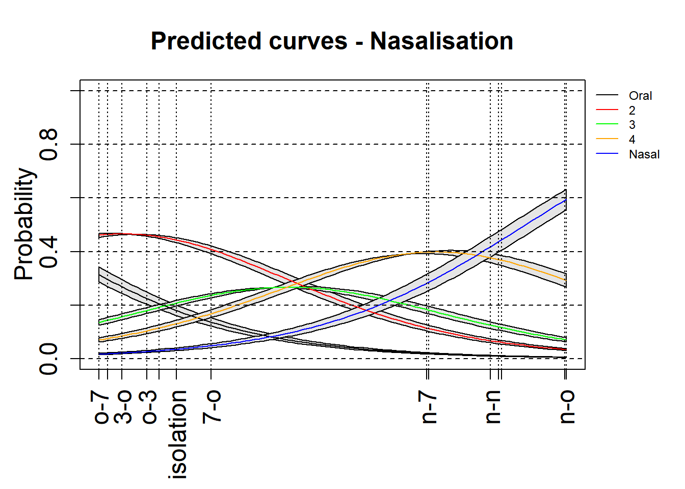
Check if the results are different between our initial model (with clm) and our new model (with clmm).
4.5.2 Subjective estimates of the weight of the referents of 81 English nouns.
This dataset comes from the LanguageR package. It contains the subjective estimates of the weight of the referents of 81 English nouns.
This dataset is a little complex. Data comes from multiple subjects who rated 81 nouns. The nouns are from a a class of animals and plants. The subjects are either males or females.
We can model it in various ways. Here we decided to explore whether the ratings given to a particular word are different, when the class is either animal or a plant and if males rated the nouns differently from males. We will only use subject as a random effect. We also model the contribution of frequency.
4.5.2.1 Importing and pre-processing
weightRatings <- weightRatings %>%
  mutate(Rating = factor(Rating),
         Subject = factor(Subject),
         Sex = factor(Sex),
         Word = factor(Word),
         Class = factor(Class))
weightRatings %>%
  head(10)
## Subject Rating Trial Sex Word Frequency Class
## 1 A1 5 1 F horse 7.771910 animal
## 2 A1 1 2 F gherkin 2.079442 plant
## 3 A1 3 3 F hedgehog 3.637586 animal
## 4 A1 1 4 F bee 5.700444 animal
## 5 A1 1 5 F peanut 4.595120 plant
## 6 A1 2 6 F pear 4.727388 plant
## 7 A1 3 7 F pineapple 3.988984 plant
## 8 A1 2 8 F frog 5.129899 animal
## 9 A1 1 9 F blackberry 4.060443 plant
## 10 A1 3 10 F pigeon 5.262690 animal4.5.2.2 Model specifications
4.5.2.2.1 No random effects
We run our first clm model as a simple, i.e., with no random effects
##    user  system elapsed
## 0.11 0.10 0.05## formula: Response ~ Context
## data: .
##
## link threshold nobs logLik AIC niter max.grad cond.H
## logit flexible 405 -526.16 1086.31 5(0) 3.61e-09 1.3e+02
##
## Coefficients:
## Estimate Std. Error z value Pr(>|z|)
## Context3--3 -0.1384 0.5848 -0.237 0.8130
## Context3-n 3.5876 0.4721 7.600 2.96e-14 ***
## Context3-o -0.4977 0.3859 -1.290 0.1971
## Context7-n 2.3271 0.5079 4.582 4.60e-06 ***
## Context7-o 0.2904 0.4002 0.726 0.4680
## Contextn-3 2.8957 0.6685 4.331 1.48e-05 ***
## Contextn-7 2.2678 0.4978 4.556 5.22e-06 ***
## Contextn-n 2.8697 0.4317 6.647 2.99e-11 ***
## Contextn-o 3.5152 0.4397 7.994 1.30e-15 ***
## Contexto-3 -0.2540 0.4017 -0.632 0.5272
## Contexto-7 -0.6978 0.3769 -1.851 0.0641 .
## Contexto-n 2.9640 0.4159 7.126 1.03e-12 ***
## Contexto-o -0.6147 0.3934 -1.562 0.1182
## ---
## Signif. codes: 0 '***' 0.001 '**' 0.01 '*' 0.05 '.' 0.1 ' ' 1
##
## Threshold coefficients:
## Estimate Std. Error z value
## 1|2 -1.4615 0.2065 -7.077
## 2|3 0.4843 0.1824 2.655
## 3|4 1.5492 0.2044 7.578
## 4|5 3.1817 0.2632 12.0894.5.2.2.2 Random effects 1 - Intercepts only
We run our first model as a simple, i.e., with random intercepts
system.time(mdl.clmm.Int.1 <- weightRatings %>%
  clmm(Rating ~ Class * Sex  * Frequency + (1|Subject:Word), data = .))
## user system elapsed
## 9.23 0.12 9.36## Cumulative Link Mixed Model fitted with the Laplace approximation
##
## formula: Response ~ Context + (1 | Subject) + (1 | Item)
## data: .
##
## link threshold nobs logLik AIC niter max.grad cond.H
## logit flexible 405 -520.89 1079.79 1395(2832) 7.26e-04 1.2e+02
##
## Random effects:
## Groups Name Variance Std.Dev.
## Item (Intercept) 1.272e-14 1.128e-07
## Subject (Intercept) 1.942e-01 4.407e-01
## Number of groups: Item 45, Subject 9
##
## Coefficients:
## Estimate Std. Error z value Pr(>|z|)
## Context3--3 -0.1634 0.5798 -0.282 0.7781
## Context3-n 3.6779 0.4804 7.657 1.91e-14 ***
## Context3-o -0.5156 0.3873 -1.331 0.1831
## Context7-n 2.3775 0.5185 4.585 4.54e-06 ***
## Context7-o 0.3279 0.4046 0.810 0.4177
## Contextn-3 3.0361 0.6677 4.547 5.43e-06 ***
## Contextn-7 2.3599 0.4925 4.792 1.65e-06 ***
## Contextn-n 2.9633 0.4339 6.830 8.52e-12 ***
## Contextn-o 3.6644 0.4495 8.153 3.56e-16 ***
## Contexto-3 -0.2772 0.4000 -0.693 0.4883
## Contexto-7 -0.7334 0.3800 -1.930 0.0536 .
## Contexto-n 3.0672 0.4220 7.268 3.65e-13 ***
## Contexto-o -0.6505 0.4015 -1.620 0.1052
## ---
## Signif. codes: 0 '***' 0.001 '**' 0.01 '*' 0.05 '.' 0.1 ' ' 1
##
## Threshold coefficients:
## Estimate Std. Error z value
## 1|2 -1.5141 0.2554 -5.928
## 2|3 0.5077 0.2358 2.153
## 3|4 1.6039 0.2538 6.319
## 4|5 3.2921 0.3072 10.7184.5.2.2.3 Random effects 2 - Intercepts and Slopes
We run our second model as a simple, i.e., with random intercepts and random slopes for subject by class.
system.time(mdl.clmm.Slope.1 <- weightRatings %>%
  clmm(Rating ~ Class * Sex  * Frequency + (Class|Subject:Word), data = .))
## user system elapsed
## 22.78 1.14 24.11## Cumulative Link Mixed Model fitted with the Laplace approximation
##
## formula: Response ~ Context + (Context | Subject) + (1 | Item)
## data: .
##
## link threshold nobs logLik AIC niter max.grad cond.H
## logit flexible 405 -492.53 1231.05 55305(218422) 8.87e-02 1.5e+04
##
## Random effects:
## Groups Name Variance Std.Dev. Corr
## Item (Intercept) 0.05939 0.2437
## Subject (Intercept) 0.70845 0.8417
## Context3--3 2.34447 1.5312 -0.755
## Context3-n 4.43319 2.1055 -0.258 0.654
## Context3-o 1.37733 1.1736 -0.677 0.985 0.649
## Context7-n 4.33218 2.0814 -0.544 0.729 0.389 0.709
## Context7-o 1.55843 1.2484 -0.809 0.740 0.068 0.682 0.431
## Contextn-3 7.99273 2.8271 -0.251 0.725 0.807 0.773 0.204
## Contextn-7 4.87737 2.2085 -0.276 0.563 0.516 0.553 -0.090
## Contextn-n 3.60679 1.8992 -0.659 0.924 0.662 0.916 0.420
## Contextn-o 2.26056 1.5035 -0.730 0.633 0.022 0.615 0.141
## Contexto-3 1.00547 1.0027 -0.159 0.484 0.443 0.513 -0.189
## Contexto-7 1.48508 1.2186 -0.889 0.738 0.196 0.637 0.456
## Contexto-n 2.76687 1.6634 -0.874 0.871 0.398 0.787 0.578
## Contexto-o 1.78059 1.3344 -0.883 0.645 0.300 0.547 0.739
##
##
##
##
##
##
##
##
## 0.336
## 0.547 0.824
## 0.744 0.867 0.825
## 0.915 0.429 0.639 0.747
## 0.457 0.840 0.969 0.771 0.626
## 0.946 0.290 0.511 0.721 0.811 0.359
## 0.919 0.469 0.581 0.837 0.769 0.434 0.970
## 0.561 0.031 -0.057 0.411 0.345 -0.221 0.723 0.733
## Number of groups: Item 45, Subject 9
##
## Coefficients:
## Estimate Std. Error z value Pr(>|z|)
## Context3--3 -0.2625 0.8280 -0.317 0.75120
## Context3-n 4.6025 0.9754 4.718 2.38e-06 ***
## Context3-o -0.5739 0.5821 -0.986 0.32413
## Context7-n 2.5260 0.9164 2.756 0.00584 **
## Context7-o 0.3748 0.6183 0.606 0.54433
## Contextn-3 4.1834 1.4119 2.963 0.00305 **
## Contextn-7 2.9393 0.9457 3.108 0.00188 **
## Contextn-n 3.5724 0.8166 4.375 1.21e-05 ***
## Contextn-o 4.4321 0.7515 5.898 3.69e-09 ***
## Contexto-3 -0.3567 0.5562 -0.641 0.52138
## Contexto-7 -0.8254 0.5861 -1.408 0.15905
## Contexto-n 3.6329 0.7410 4.903 9.44e-07 ***
## Contexto-o -0.6508 0.6248 -1.042 0.29755
## ---
## Signif. codes: 0 '***' 0.001 '**' 0.01 '*' 0.05 '.' 0.1 ' ' 1
##
## Threshold coefficients:
## Estimate Std. Error z value
## 1|2 -1.7147 0.3662 -4.682
## 2|3 0.5701 0.3481 1.638
## 3|4 1.8427 0.3666 5.026
## 4|5 3.9828 0.4399 9.0544.5.2.3 Testing significance
We can evaluate whether “Context” improves the model fit, by comparing a null model with our model. Of course “Context” is improving the model fit.
4.5.2.3.1 Null vs no random
## Likelihood ratio tests of cumulative link models:
##
##                formula:                         link: threshold:
## mdl.clm.Null.1 Rating ~ 1                       logit flexible
## mdl.clm.1      Rating ~ Class * Sex * Frequency logit flexible
##
##                no.par    AIC  logLik LR.stat df Pr(>Chisq)
## mdl.clm.Null.1      6 5430.2 -2709.1
## mdl.clm.1          13 4800.2 -2387.1  644.05  7  < 2.2e-16 ***
## ---
## Signif. codes:  0 '***' 0.001 '**' 0.01 '*' 0.05 '.' 0.1 ' ' 1
4.5.2.3.2 No random vs Random Intercepts
## Likelihood ratio tests of cumulative link models:
##
##                formula:                                              link:
## mdl.clm.1      Rating ~ Class * Sex * Frequency                      logit
## mdl.clmm.Int.1 Rating ~ Class * Sex * Frequency + (1 | Subject:Word) logit
##                threshold:
## mdl.clm.1      flexible
## mdl.clmm.Int.1 flexible
##
##                no.par    AIC  logLik LR.stat df Pr(>Chisq)
## mdl.clm.1          13 4800.2 -2387.1
## mdl.clmm.Int.1     14 4801.5 -2386.8  0.6612  1     0.4161
4.5.2.3.3 Random Intercepts vs Random Slope
## Likelihood ratio tests of cumulative link models:
##
##                  formula:
## mdl.clmm.Int.1   Rating ~ Class * Sex * Frequency + (1 | Subject:Word)
## mdl.clmm.Slope.1 Rating ~ Class * Sex * Frequency + (Class | Subject:Word)
##                  link: threshold:
## mdl.clmm.Int.1   logit flexible
## mdl.clmm.Slope.1 logit flexible
##
##                  no.par    AIC  logLik LR.stat df Pr(>Chisq)
## mdl.clmm.Int.1       14 4801.5 -2386.8
## mdl.clmm.Slope.1     16 4789.3 -2378.7  16.194  2  0.0003045 ***
## ---
## Signif. codes:  0 '***' 0.001 '**' 0.01 '*' 0.05 '.' 0.1 ' ' 1
The model comparison above shows that using random intercepts is enough in our case. By subject Random Slopes are not needed; subjects “seem” to show similarities in how they produced the items.
4.5.2.4 Model’s fit
print(tab_model(mdl.clmm.Int.1, file = paste0("outputs/mdl.clmm.Int.1.html")))
htmltools::includeHTML("outputs/mdl.clmm.Int.1.html")| Rating | |||
|---|---|---|---|
| Predictors | Odds Ratios | CI | p |
| 1|2 | 0.42 | 0.35 – 0.49 | <0.001 |
| 2|3 | 1.75 | 1.54 – 2.00 | <0.001 |
| 3|4 | 4.65 | 4.13 – 5.24 | <0.001 |
| 4|5 | 9.54 | 8.54 – 10.67 | <0.001 |
| 5|6 | 22.39 | 22.38 – 22.40 | <0.001 |
| 6|7 | 50.41 | 50.39 – 50.43 | <0.001 |
| Class [plant] | 0.31 | 0.16 – 0.60 | <0.001 |
| Sex [M] | 0.50 | 0.50 – 0.50 | <0.001 |
| Frequency | 1.27 | 1.27 – 1.27 | <0.001 |
| Class [plant] × Sex [M] | 1.46 | 0.43 – 4.93 | 0.545 |
| Class [plant] × Frequency | 0.76 | 0.66 – 0.88 | <0.001 |
| Sex [M] × Frequency | 1.08 | 1.08 – 1.08 | <0.001 |
| (Class [plant] × Sex [M]) × Frequency |
0.92 | 0.70 – 1.21 | 0.563 |
| N Subject | 20 | ||
| N Word | 81 | ||
| Observations | 1620 | ||
4.5.2.5 Interpreting a cumulative model
As a way to interpret the model, we can look at the coefficients and make sense of the results. A CLM model is a Logistic model with a cumulative effect. The “Coefficients” are the estimates for each level of the fixed effect; the “Threshold coefficients” are those of the response. For the former, a negative coefficient indicates a negative association with the response; and a positive is positively associated with the response. The p values are indicating the significance of each level. For the “Threshold coefficients”, we can see the cumulative effects of ratings 1|2, 2|3, 3|4 and 4|5 which indicate an overall increase in the ratings from 1 to 5.
4.5.2.6 Plotting
4.5.2.6.1 No confidence intervals
We use a modified version of a plotting function that allows us to visualise the effects. For this, we use the base R plotting functions. The version below is without confidence intervals.
par(oma = c(4, 0, 0, 3), mgp = c(2, 1, 0))
xlim  =  c(min(mdl.clmm.Int.1$beta), max(mdl.clmm.Int.1$beta))
ylim  =  c(0, 1)
plot(0, 0, xlim = xlim, ylim = ylim, type = "n", ylab = expression(Probability), xlab = "", xaxt = "n", main = "Predicted curves", cex = 2, cex.lab = 1.5, cex.main = 1.5, cex.axis = 1.5)
axis(side = 1, at = mdl.clmm.Int.1$beta, labels = names(mdl.clmm.Int.1$beta), las = 2, cex = 0.75, cex.lab = 0.75, cex.axis = 0.75)
xs  =  seq(xlim[1], xlim[2], length.out = 100)
lines(xs, plogis(mdl.clmm.Int.1$Theta[1] - xs), col = 'black')
lines(xs, plogis(mdl.clmm.Int.1$Theta[2] - xs) - plogis(mdl.clmm.Int.1$Theta[1] - xs), col = 'red')
lines(xs, plogis(mdl.clmm.Int.1$Theta[3] - xs) - plogis(mdl.clmm.Int.1$Theta[2] - xs), col = 'green')
lines(xs, plogis(mdl.clmm.Int.1$Theta[4] - xs) - plogis(mdl.clmm.Int.1$Theta[3] - xs), col = 'orange')
lines(xs, plogis(mdl.clmm.Int.1$Theta[5] - xs) - plogis(mdl.clmm.Int.1$Theta[4] - xs), col = 'yellow')
lines(xs, plogis(mdl.clmm.Int.1$Theta[6] - xs) - plogis(mdl.clmm.Int.1$Theta[5] - xs), col = 'grey')
lines(xs, 1 - (plogis(mdl.clmm.Int.1$Theta[6] - xs)), col = 'blue')
abline(v = c(0,mdl.clmm.Int.1$beta),lty = 3)
abline(h = 0, lty = "dashed")
abline(h = 0.2, lty = "dashed")
abline(h = 0.4, lty = "dashed")
abline(h = 0.6, lty = "dashed")
abline(h = 0.8, lty = "dashed")
abline(h = 1, lty = "dashed")

legend(par('usr')[2], par('usr')[4], bty = 'n', xpd = NA, lty = 1,
       col = c("black", "red", "green", "orange", "yellow", "grey", "blue"),
       legend = c("1", "2", "3", "4", "5", "6", "7"), cex = 0.75)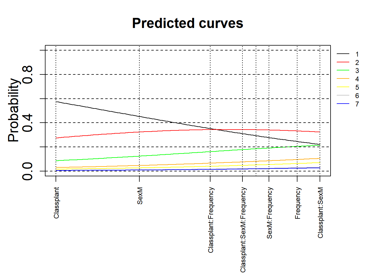
4.5.2.6.2 With confidence intervals
Here is an attempt to add the 97.5% confidence intervals to these plots. This is an experimental attempt and any feedback is welcome!
par(oma = c(4, 0, 0, 3), mgp = c(2, 1, 0))
xlim  =  c(min(mdl.clmm.Int.1$beta), max(mdl.clmm.Int.1$beta))
ylim  =  c(0, 1)
plot(0, 0, xlim = xlim, ylim = ylim, type = "n", ylab = expression(Probability), xlab = "", xaxt = "n", main = "Predicted curves", cex = 2, cex.lab = 1.5, cex.main = 1.5, cex.axis = 1.5)
axis(side = 1, at = mdl.clmm.Int.1$beta, labels = names(mdl.clmm.Int.1$beta), las = 2, cex = 0.75, cex.lab = 0.75, cex.axis = 0.75)
xs  =  seq(xlim[1], xlim[2], length.out = 100)


#+CI
lines(xs, plogis(mdl.clmm.Int.1$Theta[1]+(summary(mdl.clmm.Int.1)$coefficient[,2][[1]]/1.96) - xs), col='black')
lines(xs, plogis(mdl.clmm.Int.1$Theta[2]+(summary(mdl.clmm.Int.1)$coefficient[,2][[2]]/1.96) - xs)-plogis(mdl.clmm.Int.1$Theta[1]+(summary(mdl.clmm.Int.1)$coefficient[,2][[1]]/1.96) - xs), col='red')
lines(xs, plogis(mdl.clmm.Int.1$Theta[3]+(summary(mdl.clmm.Int.1)$coefficient[,2][[3]]/1.96) - xs)-plogis(mdl.clmm.Int.1$Theta[2]+(summary(mdl.clmm.Int.1)$coefficient[,2][[2]]/1.96) - xs), col='green')
lines(xs, plogis(mdl.clmm.Int.1$Theta[4]+(summary(mdl.clmm.Int.1)$coefficient[,2][[4]]/1.96) - xs)-plogis(mdl.clmm.Int.1$Theta[3]+(summary(mdl.clmm.Int.1)$coefficient[,2][[3]]/1.96) - xs), col='orange')
lines(xs, plogis(mdl.clmm.Int.1$Theta[5]-(summary(mdl.clmm.Int.1)$coefficient[,2][[5]]/1.96) - xs)-plogis(mdl.clmm.Int.1$Theta[4]-(summary(mdl.clmm.Int.1)$coefficient[,2][[4]]/1.96) - xs), col='yellow')
lines(xs, plogis(mdl.clmm.Int.1$Theta[6]-(summary(mdl.clmm.Int.1)$coefficient[,2][[6]]/1.96) - xs)-plogis(mdl.clmm.Int.1$Theta[5]-(summary(mdl.clmm.Int.1)$coefficient[,2][[5]]/1.96) - xs), col='grey')
lines(xs, 1-(plogis(mdl.clmm.Int.1$Theta[6]-(summary(mdl.clmm.Int.1)$coefficient[,2][[6]]/1.96) - xs)), col='blue')

#-CI
lines(xs, plogis(mdl.clmm.Int.1$Theta[1]-(summary(mdl.clmm.Int.1)$coefficient[,2][[1]]/1.96) - xs), col='black')
lines(xs, plogis(mdl.clmm.Int.1$Theta[2]-(summary(mdl.clmm.Int.1)$coefficient[,2][[2]]/1.96) - xs)-plogis(mdl.clmm.Int.1$Theta[1]-(summary(mdl.clmm.Int.1)$coefficient[,2][[1]]/1.96) - xs), col='red')
lines(xs, plogis(mdl.clmm.Int.1$Theta[3]-(summary(mdl.clmm.Int.1)$coefficient[,2][[3]]/1.96) - xs)-plogis(mdl.clmm.Int.1$Theta[2]-(summary(mdl.clmm.Int.1)$coefficient[,2][[2]]/1.96) - xs), col='green')
lines(xs, plogis(mdl.clmm.Int.1$Theta[4]-(summary(mdl.clmm.Int.1)$coefficient[,2][[4]]/1.96) - xs)-plogis(mdl.clmm.Int.1$Theta[3]-(summary(mdl.clmm.Int.1)$coefficient[,2][[3]]/1.96) - xs), col='orange')
lines(xs, plogis(mdl.clmm.Int.1$Theta[5]-(summary(mdl.clmm.Int.1)$coefficient[,2][[5]]/1.96) - xs)-plogis(mdl.clmm.Int.1$Theta[4]-(summary(mdl.clmm.Int.1)$coefficient[,2][[4]]/1.96) - xs), col='yellow')
lines(xs, plogis(mdl.clmm.Int.1$Theta[6]-(summary(mdl.clmm.Int.1)$coefficient[,2][[6]]/1.96) - xs)-plogis(mdl.clmm.Int.1$Theta[5]-(summary(mdl.clmm.Int.1)$coefficient[,2][[5]]/1.96) - xs), col='grey')
lines(xs, 1-(plogis(mdl.clmm.Int.1$Theta[6]-(summary(mdl.clmm.Int.1)$coefficient[,2][[6]]/1.96) - xs)), col='blue')

## fill area around CI using c(x, rev(x)), c(y2, rev(y1))
polygon(c(xs, rev(xs)),
        c(plogis(mdl.clmm.Int.1$Theta[1]+(summary(mdl.clmm.Int.1)$coefficient[,2][[1]]/1.96) - xs), rev(plogis(mdl.clmm.Int.1$Theta[1]-(summary(mdl.clmm.Int.1)$coefficient[,2][[1]]/1.96) - xs))), col = "gray90")

polygon(c(xs, rev(xs)),
        c(plogis(mdl.clmm.Int.1$Theta[2]+(summary(mdl.clmm.Int.1)$coefficient[,2][[2]]/1.96) - xs)-plogis(mdl.clmm.Int.1$Theta[1]+(summary(mdl.clmm.Int.1)$coefficient[,2][[1]]/1.96) - xs), rev(plogis(mdl.clmm.Int.1$Theta[2]-(summary(mdl.clmm.Int.1)$coefficient[,2][[2]]/1.96) - xs)-plogis(mdl.clmm.Int.1$Theta[1]-(summary(mdl.clmm.Int.1)$coefficient[,2][[1]]/1.96) - xs))), col = "gray90")


polygon(c(xs, rev(xs)),
        c(plogis(mdl.clmm.Int.1$Theta[3]+(summary(mdl.clmm.Int.1)$coefficient[,2][[3]]/1.96) - xs)-plogis(mdl.clmm.Int.1$Theta[2]+(summary(mdl.clmm.Int.1)$coefficient[,2][[2]]/1.96) - xs), rev(plogis(mdl.clmm.Int.1$Theta[3]-(summary(mdl.clmm.Int.1)$coefficient[,2][[3]]/1.96) - xs)-plogis(mdl.clmm.Int.1$Theta[2]-(summary(mdl.clmm.Int.1)$coefficient[,2][[2]]/1.96) - xs))), col = "gray90")

polygon(c(xs, rev(xs)),
        c(plogis(mdl.clmm.Int.1$Theta[4]+(summary(mdl.clmm.Int.1)$coefficient[,2][[4]]/1.96) - xs)-plogis(mdl.clmm.Int.1$Theta[3]+(summary(mdl.clmm.Int.1)$coefficient[,2][[3]]/1.96) - xs), rev(plogis(mdl.clmm.Int.1$Theta[4]-(summary(mdl.clmm.Int.1)$coefficient[,2][[4]]/1.96) - xs)-plogis(mdl.clmm.Int.1$Theta[3]-(summary(mdl.clmm.Int.1)$coefficient[,2][[3]]/1.96) - xs))), col = "gray90")

polygon(c(xs, rev(xs)),
        c(plogis(mdl.clmm.Int.1$Theta[5]+(summary(mdl.clmm.Int.1)$coefficient[,2][[5]]/1.96) - xs)-plogis(mdl.clmm.Int.1$Theta[4]+(summary(mdl.clmm.Int.1)$coefficient[,2][[4]]/1.96) - xs), rev(plogis(mdl.clmm.Int.1$Theta[5]-(summary(mdl.clmm.Int.1)$coefficient[,2][[5]]/1.96) - xs)-plogis(mdl.clmm.Int.1$Theta[4]-(summary(mdl.clmm.Int.1)$coefficient[,2][[4]]/1.96) - xs))), col = "gray90")

polygon(c(xs, rev(xs)),
        c(plogis(mdl.clmm.Int.1$Theta[6]+(summary(mdl.clmm.Int.1)$coefficient[,2][[6]]/1.96) - xs)-plogis(mdl.clmm.Int.1$Theta[5]+(summary(mdl.clmm.Int.1)$coefficient[,2][[5]]/1.96) - xs), rev(plogis(mdl.clmm.Int.1$Theta[6]-(summary(mdl.clmm.Int.1)$coefficient[,2][[6]]/1.96) - xs)-plogis(mdl.clmm.Int.1$Theta[5]-(summary(mdl.clmm.Int.1)$coefficient[,2][[5]]/1.96) - xs))), col = "gray90")


polygon(c(xs, rev(xs)),
        c(1-(plogis(mdl.clmm.Int.1$Theta[6]-(summary(mdl.clmm.Int.1)$coefficient[,2][[6]]/1.96) - xs)), rev(1-(plogis(mdl.clmm.Int.1$Theta[6]+(summary(mdl.clmm.Int.1)$coefficient[,2][[6]]/1.96) - xs)))), col = "gray90")


lines(xs, plogis(mdl.clmm.Int.1$Theta[1] - xs), col = 'black')
lines(xs, plogis(mdl.clmm.Int.1$Theta[2] - xs) - plogis(mdl.clmm.Int.1$Theta[1] - xs), col = 'red')
lines(xs, plogis(mdl.clmm.Int.1$Theta[3] - xs) - plogis(mdl.clmm.Int.1$Theta[2] - xs), col = 'green')
lines(xs, plogis(mdl.clmm.Int.1$Theta[4] - xs) - plogis(mdl.clmm.Int.1$Theta[3] - xs), col = 'orange')
lines(xs, plogis(mdl.clmm.Int.1$Theta[5] - xs) - plogis(mdl.clmm.Int.1$Theta[4] - xs), col = 'yellow')
lines(xs, plogis(mdl.clmm.Int.1$Theta[6] - xs) - plogis(mdl.clmm.Int.1$Theta[5] - xs), col = 'grey')
lines(xs, 1 - (plogis(mdl.clmm.Int.1$Theta[6] - xs)), col = 'blue')
abline(v = c(0,mdl.clmm.Int.1$beta),lty = 3)
abline(h = 0, lty = "dashed")
abline(h = 0.2, lty = "dashed")
abline(h = 0.4, lty = "dashed")
abline(h = 0.6, lty = "dashed")
abline(h = 0.8, lty = "dashed")
abline(h = 1, lty = "dashed")

legend(par('usr')[2], par('usr')[4], bty = 'n', xpd = NA, lty = 1,
       col = c("black", "red", "green", "orange", "yellow", "grey", "blue"),
       legend = c("1", "2", "3", "4", "5", "6", "7"), cex = 0.75)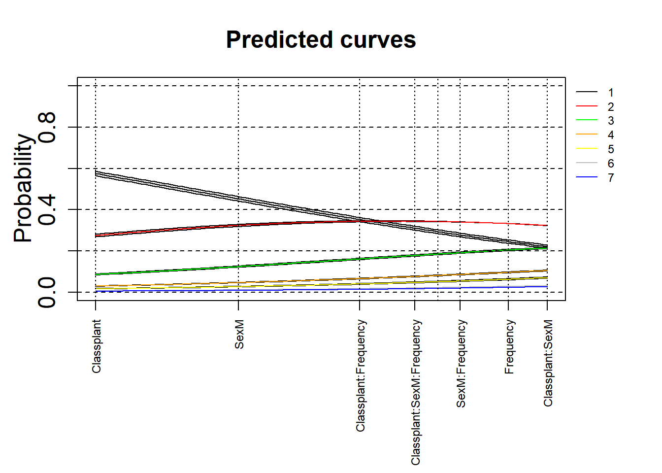
Check if the results are different between our initial model (with clm) and our new model (with clmm).