4.3 Linear Mixed-effects Models. Why random effects matter

Let’s generate a new dataframe that we will use later on for our mixed models

We will use the faux package. It is available on CRAN, but it is possible that it is not available for your version of R (I used version 4.5). In this case, you need to install it via github. The package faux is a package that allows you to simulate data for your experiments. It is a very useful package to test your ideas and to assess the impact of particular predictors on your dependant variable.

To install it, you will first need to install the package devtools, and then install the package faux using the function devtools::install_github. Uncomment the code chunk below

# install.packages("devtools")
# devtools::install_github("debruine/faux")
# library(faux)

4.3.1 Dataframe (simulated)

Our experiment has the following structure: we asked 40 subjects to respond to 40 items in a fully crossed design. There were two IVs: Condition with congruent and incongruent and Age with young and old. The Condition is a within subject variable; age is a between subject. However, Condition and Age were both within item variables. The dependant variable was LookingTime.

This meant that we used items within each of the young and the old subjects in addition to items within each of the congurent and incongruent conditions.

Our research question is as follows: Age of subject will impact the Looking Time in the two conditions. Our hypothesis is: The older a subject is, the more the looking time it is to the incongruent condition.

We will use the package faux to simulate a dataframe. This step is crucial in assessing contributions of particular predictors and for testing ideas as we already know the distribution of the data and what to expect as an outcome when it comes to the fixed effect in question.

The simulated data has the following parameters

set.seed(42)
# define parameters
Subj_n = 40  # number of subjects
Item_n = 40  # number of items
b0 = 100       # intercept
b1 = 2.5 * b0   # fixed effect of condition
u0s_sd = 300   # random intercept SD for subjects
u0i_sd = 200   # random intercept SD for items
u1s_sd = 100   # random b1 slope SD for subjects
u1i_sd = 50   # random b1 slope SD for items
r01s = -0.3     # correlation between random effects 0 and 1 for subjects
r01i = 0.2     # correlation between random effects 0 and 1 for items
sigma_sd = 150 # error SD

# set up data structure
dataCong <- add_random(Subj = Subj_n, Item = Item_n) %>%
  # add within categorical variable for subject
  add_within("Subj", Cond = c("Congruent", "Incongruent")) %>%
  add_recode("Cond", "Cond.Incongruent", Congruent = 0, Incongruent = 1) %>%
  # add between categorical variable for subject
  add_between("Subj", Age = c("Young", "Old")) %>%
  add_recode("Age", "Age.Old", Young = 0, Old = 1) %>%
  # add random effects 
  add_ranef("Subj", u0s = u0s_sd, u1s = u1s_sd, .cors = r01s) %>%
  add_ranef("Item", u0i = u0i_sd, u1i = u1i_sd, .cors = r01i) %>%
  ##add_ranef(c("Subj", "Item"), u0si = u0s_sd + u0i_sd) %>%
  ##add_ranef(c("Subj", "Item"), u1si = u1s_sd + u1i_sd) %>%
  add_ranef(sigma = sigma_sd) %>%
  # calculate DV
  mutate(LookingTime = b0 + b1 + u0s + u0i + #u0si + u1si +
           (((b1 + u1s) + 0.5) * Cond.Incongruent) + (((b1 + u1s) + 0.9) * Age.Old) + # subject specific variation
           (((b1 + u1i) - 0.3) * Cond.Incongruent) + (((b1 + u1i) - 0.25) * Age.Old) + # item specific variation  
           sigma)
write.csv(dataCong, "data/dataCong.csv")

If you were not able to install the faux package, simply uncomment the following line of code below to import the dataset

#dataCong <- read.csv("dataCong.csv")[-1]

4.3.1.1 Counts

dataCong <- dataCong %>% 
  mutate(Subj = factor(Subj),
         Item = factor(Item))
dataCong

## # A tibble: 3,200 × 12
##    Subj   Item   Cond    Cond.Incongruent Age   Age.Old   u0s   u1s    u0i   u1i
##    <fct>  <fct>  <fct>              <dbl> <fct>   <dbl> <dbl> <dbl>  <dbl> <dbl>
##  1 Subj01 Item01 Congru…                0 Young       0 -413.  26.2 -306.  56.9 
##  2 Subj01 Item01 Incong…                1 Young       0 -413.  26.2 -306.  56.9 
##  3 Subj01 Item02 Congru…                0 Young       0 -413.  26.2  -55.4 69.1 
##  4 Subj01 Item02 Incong…                1 Young       0 -413.  26.2  -55.4 69.1 
##  5 Subj01 Item03 Congru…                0 Young       0 -413.  26.2  -17.4 -7.03
##  6 Subj01 Item03 Incong…                1 Young       0 -413.  26.2  -17.4 -7.03
##  7 Subj01 Item04 Congru…                0 Young       0 -413.  26.2   21.6 50.0 
##  8 Subj01 Item04 Incong…                1 Young       0 -413.  26.2   21.6 50.0 
##  9 Subj01 Item05 Congru…                0 Young       0 -413.  26.2  239.  12.8 
## 10 Subj01 Item05 Incong…                1 Young       0 -413.  26.2  239.  12.8 
## # ℹ 3,190 more rows
## # ℹ 2 more variables: sigma <dbl>, LookingTime <dbl>

4.3.1.1.1 Subjects

dataCong %>% 
  group_by(Cond, Age, Subj) %>% 
  summarise(count = n())

## # A tibble: 80 × 4
## # Groups:   Cond, Age [4]
##    Cond      Age   Subj   count
##    <fct>     <fct> <fct>  <int>
##  1 Congruent Young Subj01    40
##  2 Congruent Young Subj03    40
##  3 Congruent Young Subj05    40
##  4 Congruent Young Subj07    40
##  5 Congruent Young Subj09    40
##  6 Congruent Young Subj11    40
##  7 Congruent Young Subj13    40
##  8 Congruent Young Subj15    40
##  9 Congruent Young Subj17    40
## 10 Congruent Young Subj19    40
## # ℹ 70 more rows

4.3.1.1.2 Items

4.3.1.1.3 Age

dataCong %>% 
  group_by(Age, Item) %>% 
  summarise(count = n())

## # A tibble: 80 × 3
## # Groups:   Age [2]
##    Age   Item   count
##    <fct> <fct>  <int>
##  1 Young Item01    40
##  2 Young Item02    40
##  3 Young Item03    40
##  4 Young Item04    40
##  5 Young Item05    40
##  6 Young Item06    40
##  7 Young Item07    40
##  8 Young Item08    40
##  9 Young Item09    40
## 10 Young Item10    40
## # ℹ 70 more rows

4.3.1.1.4 Cond

dataCong %>% 
  group_by(Cond, Item) %>% 
  summarise(count = n())

## # A tibble: 80 × 3
## # Groups:   Cond [2]
##    Cond      Item   count
##    <fct>     <fct>  <int>
##  1 Congruent Item01    40
##  2 Congruent Item02    40
##  3 Congruent Item03    40
##  4 Congruent Item04    40
##  5 Congruent Item05    40
##  6 Congruent Item06    40
##  7 Congruent Item07    40
##  8 Congruent Item08    40
##  9 Congruent Item09    40
## 10 Congruent Item10    40
## # ℹ 70 more rows

4.3.1.2 Visualisations

4.3.1.2.1 Condition by Age

The figure below confirms this, where we see an increase in LookingTime in the incongruent condition and oevrall, older participants show an increase in LookingTime

dataCong %>% 
  ggplot(aes(x = Cond,
             y = LookingTime,
             colour = Age)) +
  theme_bw() + 
  geom_boxplot() +
  geom_smooth(aes(as.numeric(Cond)), method = "lm")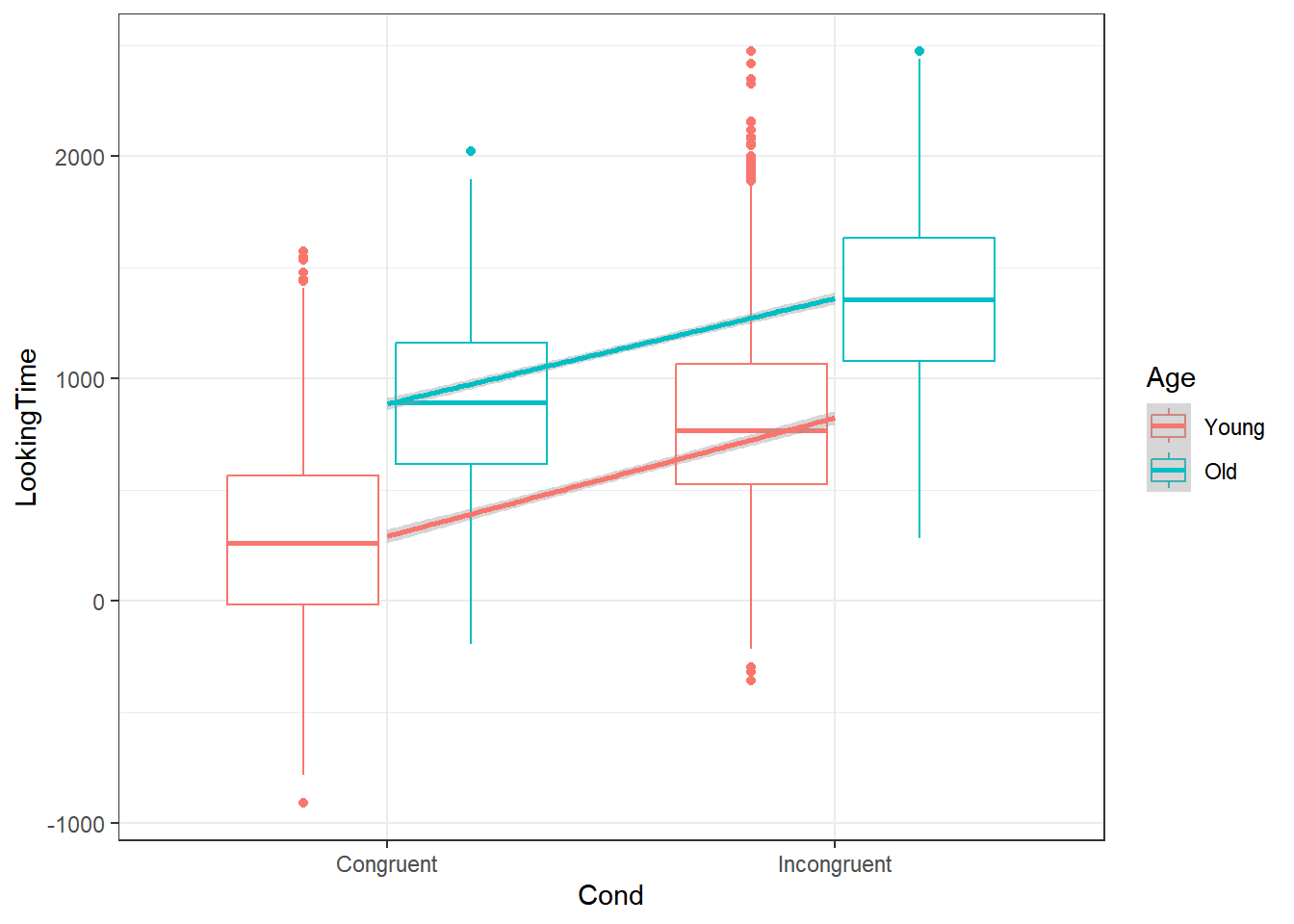

4.3.1.2.2 Subject by Condition

This figure shows that subjects are variable in how they responded to this task

dataCong %>% 
  ggplot(aes(x = Cond,
             y = LookingTime,
             colour = Subj)) +
  theme_bw() + 
  geom_point() +
  geom_smooth(aes(as.numeric(Cond)), method = "lm", se = FALSE) +
  scale_colour_manual(values = paletteer_c("grDevices::rainbow", length(unique(dataCong$Subj))))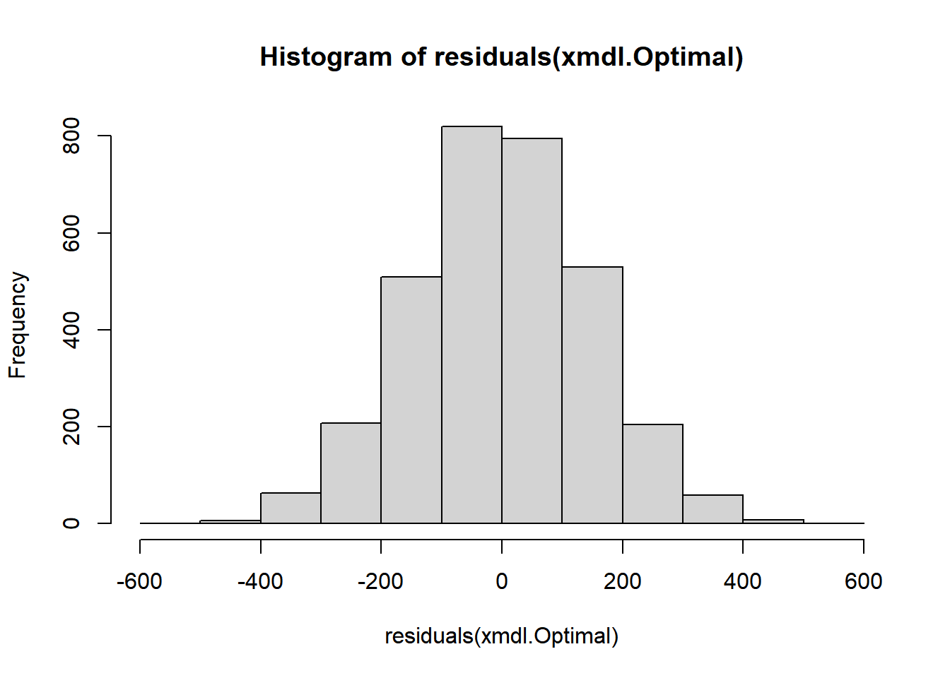

4.3.1.2.3 Subject by Age

This figure shows that subjects had an impact on the LookingTime in both age groups, simply due to their variable responses to the different items

dataCong %>% 
  ggplot(aes(x = Age,
             y = LookingTime,
             colour = Subj)) +
  theme_bw() + 
  geom_point() +
  geom_smooth(aes(as.numeric(Cond)), method = "lm", se = FALSE) +
  scale_colour_manual(values = paletteer_c("grDevices::rainbow", length(unique(dataCong$Subj))))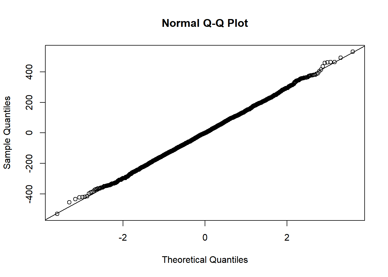

4.3.1.2.4 Item by Condition

This figure shows that items had an impact on the LookingTime in both conditions

dataCong %>% 
  ggplot(aes(x = Cond,
             y = LookingTime,
             colour = Item)) +
  theme_bw() + 
  geom_point() +
  geom_smooth(aes(as.numeric(Cond)), method = "lm", se = FALSE) +
  scale_colour_manual(values = paletteer_c("grDevices::rainbow", length(unique(dataCong$Item))))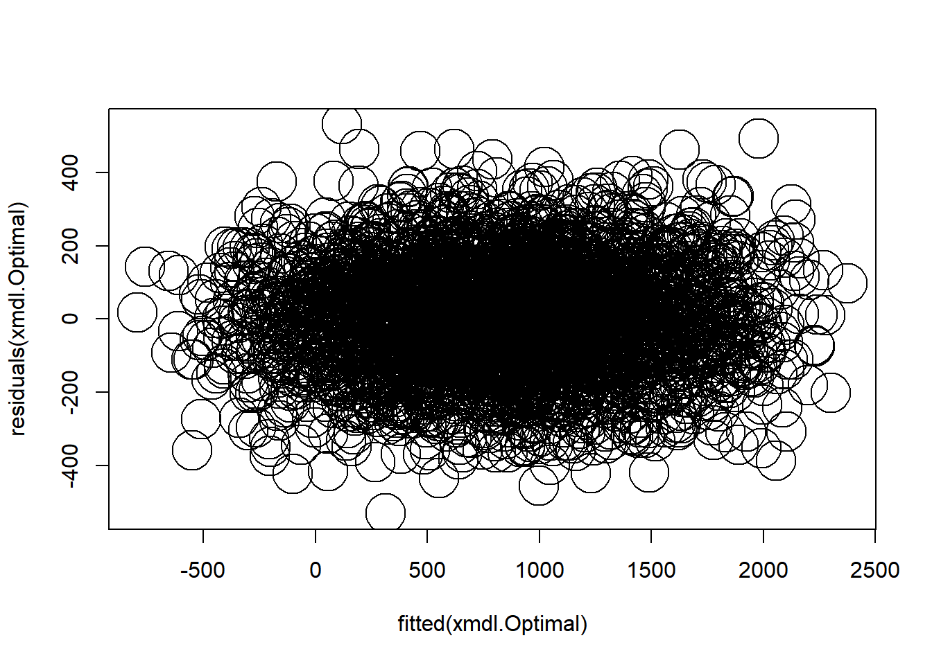

4.3.1.2.5 Subject by Age

This figure shows that items had an impact on the LookingTime in both age groups

dataCong %>% 
  ggplot(aes(x = Age,
             y = LookingTime,
             colour = Item)) +
  theme_bw() + 
  geom_point() +
  geom_smooth(aes(as.numeric(Cond)), method = "lm", se = FALSE) +
  scale_colour_manual(values = paletteer_c("grDevices::rainbow", length(unique(dataCong$Item))))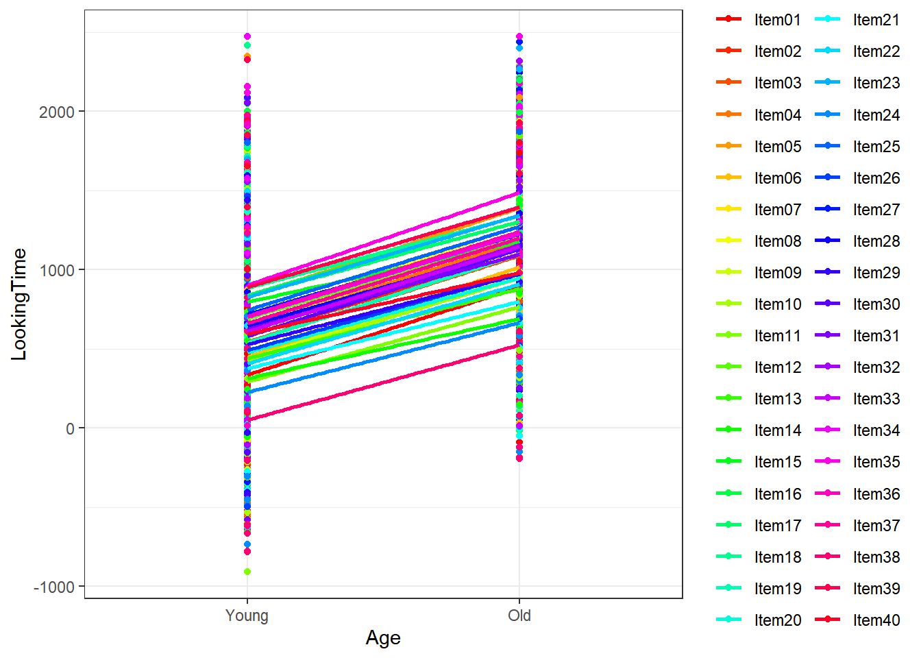

4.3.2 Modelling strategy

We use an LMER model with a crossed random effect. To choose our optimal model, we start first by a simple model with only random intercepts, increasing complexity by accounting for random slopes for both subjects and items. It is clear from our visualisation above, that there is no interaction between the two predictors. However, for demonstration purposes, we do test for this

4.3.2.1 Simple Linear Model

mdl.lm <- dataCong %>% 
  lm(LookingTime ~ Cond + Age, data = .)
summary(mdl.lm)

## 
## Call:
## lm(formula = LookingTime ~ Cond + Age, data = .)
## 
## Residuals:
##      Min       1Q   Median       3Q      Max 
## -1215.59  -290.17   -21.78   264.89  1661.41 
## 
## Coefficients:
##                 Estimate Std. Error t value Pr(>|t|)    
## (Intercept)       304.95      12.91   23.61   <2e-16 ***
## CondIncongruent   504.35      14.91   33.82   <2e-16 ***
## AgeOld            566.44      14.91   37.98   <2e-16 ***
## ---
## Signif. codes:  0 '***' 0.001 '**' 0.01 '*' 0.05 '.' 0.1 ' ' 1
## 
## Residual standard error: 421.8 on 3197 degrees of freedom
## Multiple R-squared:  0.4472, Adjusted R-squared:  0.4469 
## F-statistic:  1293 on 2 and 3197 DF,  p-value: < 2.2e-16

hist(residuals(mdl.lm))

qqnorm(residuals(mdl.lm)); qqline(residuals(mdl.lm))

plot(fitted(mdl.lm), residuals(mdl.lm), cex = 4)

4.3.2.2 No interaction

4.3.2.2.1 Crossed random intercepts

xmdl.rand.Interc <- dataCong %>% 
  lmer(LookingTime ~ Cond + Age + 
         (1 | Subj) + 
         (1 | Item), data = ., REML = FALSE,
       control = lmerControl(optimizer = "bobyqa", optCtrl = list(maxfun = 1e5)))

4.3.2.2.2 Crossed random intercepts + By-speaker random slopes

xmdl.rand.Slope1 <- dataCong %>% 
  lmer(LookingTime ~ Cond + Age + 
         (1 + Cond | Subj) + 
         (1 | Item), data = ., REML = FALSE,
       control = lmerControl(optimizer = "bobyqa", optCtrl = list(maxfun = 1e5)))

4.3.2.2.3 Crossed random intercepts + By-speaker and by-item random slopes

xmdl.rand.Slope2 <- dataCong %>% 
  lmer(LookingTime ~ Cond + Age + 
         (1 + Cond | Subj) + 
         (1 + Cond | Item), data = ., REML = FALSE,
       control = lmerControl(optimizer = "bobyqa", optCtrl = list(maxfun = 1e5)))

4.3.2.2.4 Crossed random intercepts + By-speaker and by-item random slopes

xmdl.rand.Slope3 <- dataCong %>% 
  lmer(LookingTime ~ Cond + Age + 
         (1 + Cond | Subj) + 
         (1 + Cond + Age| Item), data = ., REML = FALSE,
       control = lmerControl(optimizer = "bobyqa", optCtrl = list(maxfun = 1e5)))

4.3.2.3 With interaction

4.3.2.3.1 Crossed random intercepts + Interaction

xmdl.rand.Interc.Int <- dataCong %>% 
  lmer(LookingTime ~ Cond * Age + 
         (1 | Subj) + 
         (1 | Item), data = ., REML = FALSE,
       control = lmerControl(optimizer = "bobyqa", optCtrl = list(maxfun = 1e5)))

4.3.2.3.2 Crossed random intercepts + By-speaker random slopes + Interaction

xmdl.rand.Slope1.Int <- dataCong %>% 
  lmer(LookingTime ~ Cond * Age + 
         (1 + Cond | Subj) + 
         (1 | Item), data = ., REML = FALSE,
       control = lmerControl(optimizer = "bobyqa", optCtrl = list(maxfun = 1e5)))

4.3.2.3.3 Crossed random intercepts + By-speaker and by-item random slopes + Interaction

xmdl.rand.Slope2.Int <- dataCong %>% 
  lmer(LookingTime ~ Cond * Age + 
         (1 + Cond | Subj) + 
         (1 + Cond | Item), data = ., REML = FALSE,
       control = lmerControl(optimizer = "bobyqa", optCtrl = list(maxfun = 1e5)))

4.3.2.3.4 Crossed random intercepts + By-speaker and by-item random slopes

xmdl.rand.Slope3.Int <- dataCong %>% 
  lmer(LookingTime ~ Cond * Age + 
         (1 + Cond | Subj) + 
         (1 + Cond * Age| Item), data = ., REML = FALSE,
       control = lmerControl(optimizer = "bobyqa", optCtrl = list(maxfun = 1e5)))

4.3.2.4 Model comparison

anova(xmdl.rand.Interc, xmdl.rand.Slope1, xmdl.rand.Slope2, xmdl.rand.Slope3, xmdl.rand.Interc.Int, xmdl.rand.Slope1.Int, xmdl.rand.Slope2.Int, xmdl.rand.Slope3.Int)

## Data: .
## Models:
## xmdl.rand.Interc: LookingTime ~ Cond + Age + (1 | Subj) + (1 | Item)
## xmdl.rand.Interc.Int: LookingTime ~ Cond * Age + (1 | Subj) + (1 | Item)
## xmdl.rand.Slope1: LookingTime ~ Cond + Age + (1 + Cond | Subj) + (1 | Item)
## xmdl.rand.Slope1.Int: LookingTime ~ Cond * Age + (1 + Cond | Subj) + (1 | Item)
## xmdl.rand.Slope2: LookingTime ~ Cond + Age + (1 + Cond | Subj) + (1 + Cond | Item)
## xmdl.rand.Slope2.Int: LookingTime ~ Cond * Age + (1 + Cond | Subj) + (1 + Cond | Item)
## xmdl.rand.Slope3: LookingTime ~ Cond + Age + (1 + Cond | Subj) + (1 + Cond + Age | Item)
## xmdl.rand.Slope3.Int: LookingTime ~ Cond * Age + (1 + Cond | Subj) + (1 + Cond * Age | Item)
##                      npar   AIC   BIC logLik -2*log(L)    Chisq Df Pr(>Chisq)
## xmdl.rand.Interc        6 42074 42110 -21031     42062                       
## xmdl.rand.Interc.Int    7 42050 42093 -21018     42036  25.8359  1  3.717e-07
## xmdl.rand.Slope1        8 41834 41883 -20909     41818 217.8699  1  < 2.2e-16
## xmdl.rand.Slope1.Int    9 41833 41888 -20908     41815   3.0247  1     0.0820
## xmdl.rand.Slope2       10 41808 41869 -20894     41788  27.3253  1  1.719e-07
## xmdl.rand.Slope2.Int   11 41807 41874 -20892     41785   3.0149  1     0.0825
## xmdl.rand.Slope3       13 41780 41858 -20877     41754  31.2599  2  1.629e-07
## xmdl.rand.Slope3.Int   18 41786 41895 -20875     41750   3.3401  5     0.6477
##                         
## xmdl.rand.Interc        
## xmdl.rand.Interc.Int ***
## xmdl.rand.Slope1     ***
## xmdl.rand.Slope1.Int .  
## xmdl.rand.Slope2     ***
## xmdl.rand.Slope2.Int .  
## xmdl.rand.Slope3     ***
## xmdl.rand.Slope3.Int    
## ---
## Signif. codes:  0 '***' 0.001 '**' 0.01 '*' 0.05 '.' 0.1 ' ' 1

The results above highlight that the model accounting for both by-subject and by-item random intercepts and random slopes for Condition are improving the model fit in comparison to a more complex model. We rerun the model with REML = False

4.3.2.5 Optimal model

xmdl.Optimal <- dataCong %>% 
  lmer(LookingTime ~ Cond + Age + 
         (1 + Cond | Subj) + 
         (1 + Cond + Age | Item), data = ., REML = TRUE,
       control = lmerControl(optimizer = "bobyqa", optCtrl = list(maxfun = 1e5)))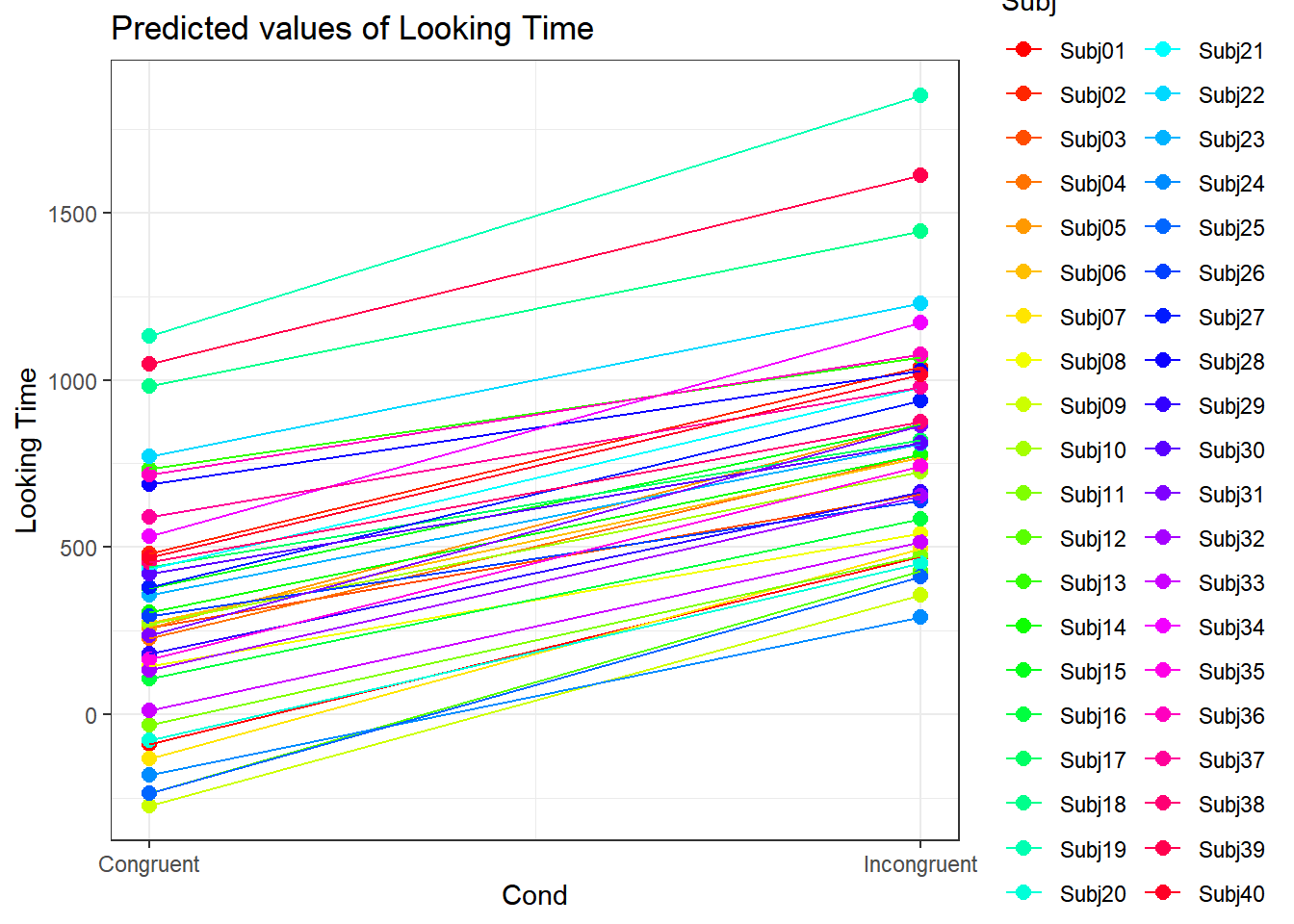

4.3.2.5.1 Model criticism

4.3.2.5.1.1 Histogram

hist(residuals(xmdl.Optimal))

4.3.2.5.1.2 QQ-plot

qqnorm(residuals(xmdl.Optimal)); qqline(residuals(xmdl.Optimal))

4.3.2.5.1.3 Residuals vs Fitted

plot(fitted(xmdl.Optimal), residuals(xmdl.Optimal), cex = 4)

4.3.2.5.2 Summary

xmdl.Optimal %>% 
  summary()

## Linear mixed model fit by REML ['lmerMod']
## Formula: LookingTime ~ Cond + Age + (1 + Cond | Subj) + (1 + Cond + Age |  
##     Item)
##    Data: .
## Control: lmerControl(optimizer = "bobyqa", optCtrl = list(maxfun = 1e+05))
## 
## REML criterion at convergence: 41724.6
## 
## Scaled residuals: 
##     Min      1Q  Median      3Q     Max 
## -3.5337 -0.6485 -0.0054  0.6647  3.5358 
## 
## Random effects:
##  Groups   Name            Variance Std.Dev. Corr       
##  Subj     (Intercept)     123480   351.40              
##           CondIncongruent  10746   103.66   -0.26      
##  Item     (Intercept)      38781   196.93              
##           CondIncongruent   1872    43.27    0.31      
##           AgeOld            1851    43.03   -0.13  0.69
##  Residual                  22613   150.38              
## Number of obs: 3200, groups:  Subj, 40; Item, 40
## 
## Fixed effects:
##                 Estimate Std. Error t value
## (Intercept)       315.04      83.42   3.777
## CondIncongruent   504.35      18.54  27.204
## AgeOld            546.28     107.70   5.072
## 
## Correlation of Fixed Effects:
##             (Intr) CndInc
## CndIncngrnt -0.120       
## AgeOld      -0.646  0.016

4.3.2.5.3 ANOVA

Anova(xmdl.Optimal)

## Analysis of Deviance Table (Type II Wald chisquare tests)
## 
## Response: LookingTime
##        Chisq Df Pr(>Chisq)    
## Cond 740.067  1  < 2.2e-16 ***
## Age   25.729  1  3.928e-07 ***
## ---
## Signif. codes:  0 '***' 0.001 '**' 0.01 '*' 0.05 '.' 0.1 ' ' 1

4.3.2.5.4 Model’s fit

print(tab_model(xmdl.Optimal, file = paste0("outputs/xmdl.Optimal.html")))
htmltools::includeHTML("outputs/xmdl.Optimal.html")

	Looking Time
Predictors	Estimates	CI	p
(Intercept)	315.04	151.48 – 478.60	<0.001
Cond [Incongruent]	504.35	468.00 – 540.70	<0.001
Age [Old]	546.28	335.12 – 757.44	<0.001
Random Effects
σ²	22612.64
τ₀₀ _Subj	123480.29
τ₀₀ _Item	38780.86
τ₁₁ _{Subj.CondIncongruent}	10745.65
τ₁₁ _{Item.CondIncongruent}	1872.30
τ₁₁ _Item.AgeOld	1851.23
ρ₀₁ _Subj	-0.26
ρ₀₁ _{Item.CondIncongruent}	0.31
ρ₀₁ _Item.AgeOld	-0.13
ICC	0.88
N _Subj	40
N _Item	40
Observations	3200
Marginal R² / Conditional R²	0.428 / 0.930

4.3.3 Plotting model’s output

4.3.3.1 With `ggstats`

We use two functions from the package ggstats.

4.3.3.1.1 A plot

ggcoef_model(xmdl.Optimal)

4.3.3.2 A plot + a table + 95% CI

ggcoef_table(xmdl.Optimal)

4.3.3.3 With `ggstatsplot`

ggcoefstats(xmdl.Optimal, point.args = list(color = paletteer_c("grDevices::rainbow", 13), stats.label.color = paletteer_c("grDevices::rainbow", 13)))

## Warning in (function (mapping = NULL, data = NULL, stat = "identity", position
## = "identity", : Ignoring unknown parameters: `stats.label.colour`

## Number of labels is greater than default palette color count.
## • Select another color `palette` (and/or `package`).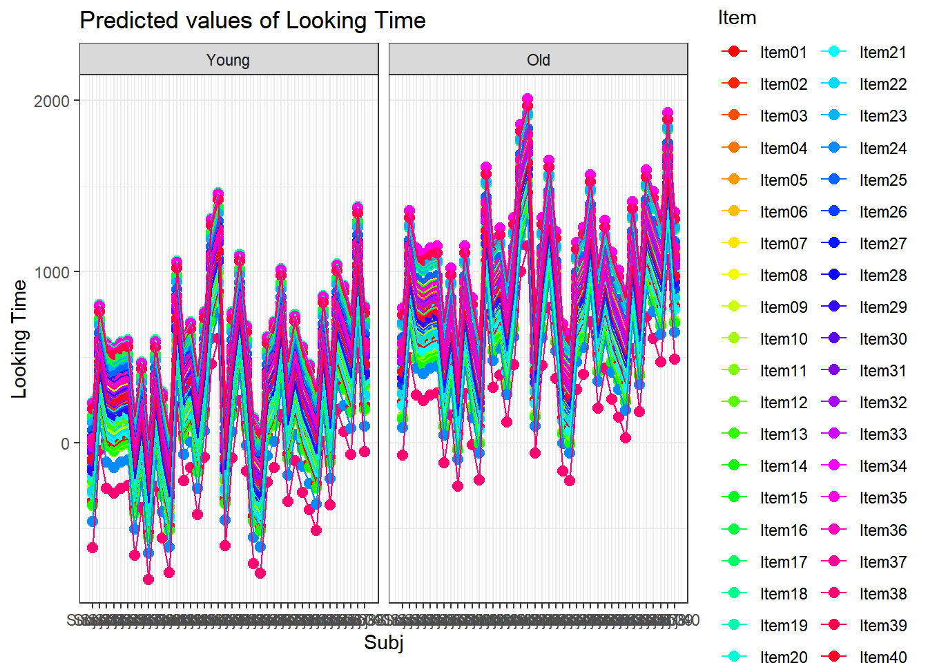

4.3.4 Exploring random effects

4.3.4.1 Subject random effects

random_effects <- ranef(xmdl.Optimal) %>%
  pluck(1) %>%
  rownames_to_column() %>%
  rename(Subject = rowname, Intercept = "(Intercept)") 
 
random_effects %>%
  knitr::kable()

Subject	Intercept	CondIncongruent
Subj01	-404.45054	58.1953368
Subj02	164.05584	56.9126271
Subj03	-56.37438	-104.0600477
Subj04	-87.06837	43.7884729
Subj05	-55.65214	104.5323900
Subj06	-42.39999	-7.1394328
Subj07	-448.81496	124.6524549
Subj08	-171.75810	-105.4504187
Subj09	-587.74594	123.6911001
Subj10	-44.50407	-50.9618431
Subj11	-346.46288	1.6396966
Subj12	-550.49633	158.6524706
Subj13	417.66027	-169.1409700
Subj14	-11.45716	-30.0008252
Subj15	62.46659	-14.3520076
Subj16	-210.03389	-23.9077430
Subj17	124.19946	-122.7635167
Subj18	666.67147	-42.1836697
Subj19	815.78333	217.1615447
Subj20	-393.58521	26.1633665
Subj21	120.64645	37.9297097
Subj22	455.31816	-46.4925696
Subj23	42.42431	-54.4053551
Subj24	-496.29436	-31.7202386
Subj25	-552.91357	144.2714898
Subj26	-21.91509	-159.7897817
Subj27	65.14521	54.5212747
Subj28	373.40089	-166.0862255
Subj29	-132.82108	-21.8820276
Subj30	104.73419	-112.8914459
Subj31	-79.72260	125.0118699
Subj32	-182.30982	15.3898936
Subj33	-303.68384	-0.1957386
Subj34	215.98609	136.5078869
Subj35	-152.60397	76.5559812
Subj36	401.50547	-145.0045141
Subj37	274.61818	-114.4122298
Subj38	139.48473	-82.7958618
Subj39	733.87830	58.5575032
Subj40	155.08935	41.5013939

4.3.4.2 Items random effects

random_effects <- ranef(xmdl.Optimal) %>%
  pluck(2) %>%
  rownames_to_column() %>%
  rename(Items = rowname, Intercept = "(Intercept)") 
 
random_effects %>%
  knitr::kable()

Items	Intercept	CondIncongruent	AgeOld
Item01	-247.414507	16.2991489	28.312990
Item02	-28.240445	20.6149279	37.267856
Item03	-27.548429	11.7099339	-3.218254
Item04	30.999046	32.2392558	32.548236
Item05	246.216859	38.0585978	2.963549
Item06	-135.583736	28.3151555	28.127356
Item07	75.461498	28.6715548	-2.095288
Item08	72.679400	69.1730999	73.479523
Item09	-180.071444	32.9237845	60.953057
Item10	-170.029328	8.4112590	23.865843
Item11	-278.857705	-39.6392919	-22.526611
Item12	114.001985	4.7652485	-15.353357
Item13	-137.533542	-49.5701246	-36.764423
Item14	-272.928912	-85.2576750	-45.340742
Item15	219.855541	-70.2475223	-83.121735
Item16	243.071753	13.0287924	-4.812872
Item17	210.792625	10.6898312	17.840004
Item18	328.737750	-36.9498461	-82.922663
Item19	-46.910049	28.2829527	22.930110
Item20	-107.870056	-25.5384308	-13.846115
Item21	-209.598744	-56.8339801	-29.482588
Item22	-190.253581	-3.0439700	20.502593
Item23	207.958662	34.4328035	33.373202
Item24	-371.211245	-46.1955836	1.751542
Item25	163.603914	15.0837752	-7.780876
Item26	-56.954235	-39.1972201	-59.652416
Item27	126.648406	7.5867262	-1.102683
Item28	48.176096	-0.4969082	1.358911
Item29	-76.699978	-27.4397677	-1.462473
Item30	-20.393146	33.1813806	36.286219
Item31	33.763413	-15.9993987	-14.400133
Item32	-15.979008	47.9237115	67.643383
Item33	64.451213	-8.2252951	-47.157817
Item34	102.286457	22.6554454	17.134672
Item35	319.882212	54.1470278	10.485257
Item36	115.886689	22.7596669	9.094458
Item37	93.471368	9.1514824	-17.490313
Item38	-523.293815	-46.1545897	-5.185309
Item39	287.858945	20.0462752	2.292928
Item40	-8.431927	-59.3622338	-34.495018

4.3.4.3 Plots

These plots below are produced with the sjPlot package.

4.3.4.3.1 Fixed effects

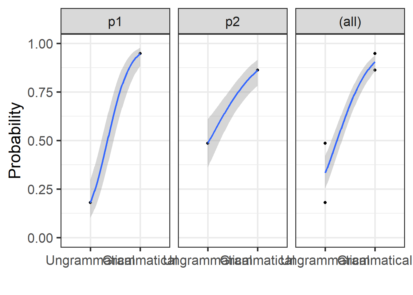
4.3.4.3.1.1 Condition

plot_model(xmdl.Optimal, type="pred", terms=c("Cond"), ci.lvl = NA, dodge = 0) + theme_bw() + geom_line()

4.3.4.3.1.2 Age

plot_model(xmdl.Optimal, type="pred", terms=c("Age"), ci.lvl = NA, dodge = 0) + theme_bw() + geom_line()

4.3.4.3.1.3 Condition by Age

plot_model(xmdl.Optimal, type="emm", terms=c("Cond", "Age"), ci.lvl = NA, dodge = 0) + theme_bw() + geom_line()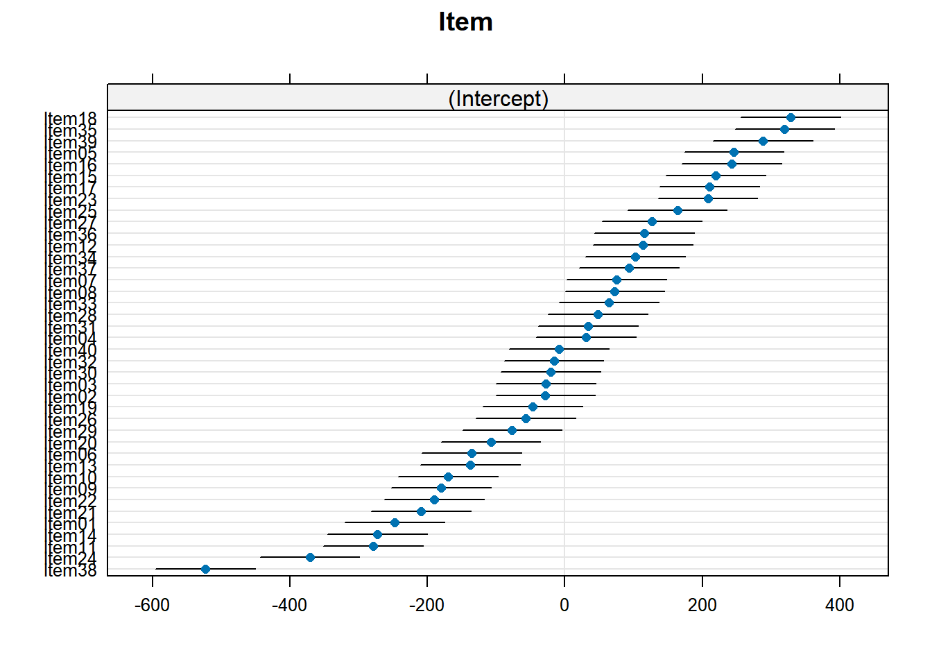

4.3.4.3.2 Random effects

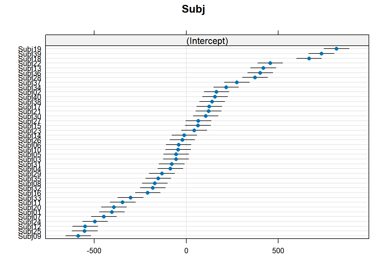
4.3.4.3.2.1 Subject

plot_model(xmdl.Optimal, type="pred", terms=c("Subj"), pred.type="re", ci.lvl = NA, dodge = 0) + theme_bw() + geom_line()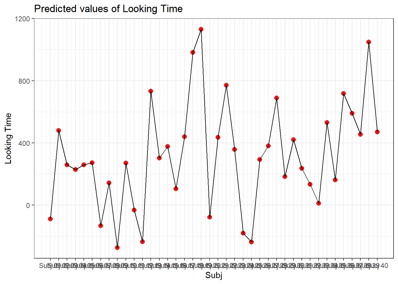

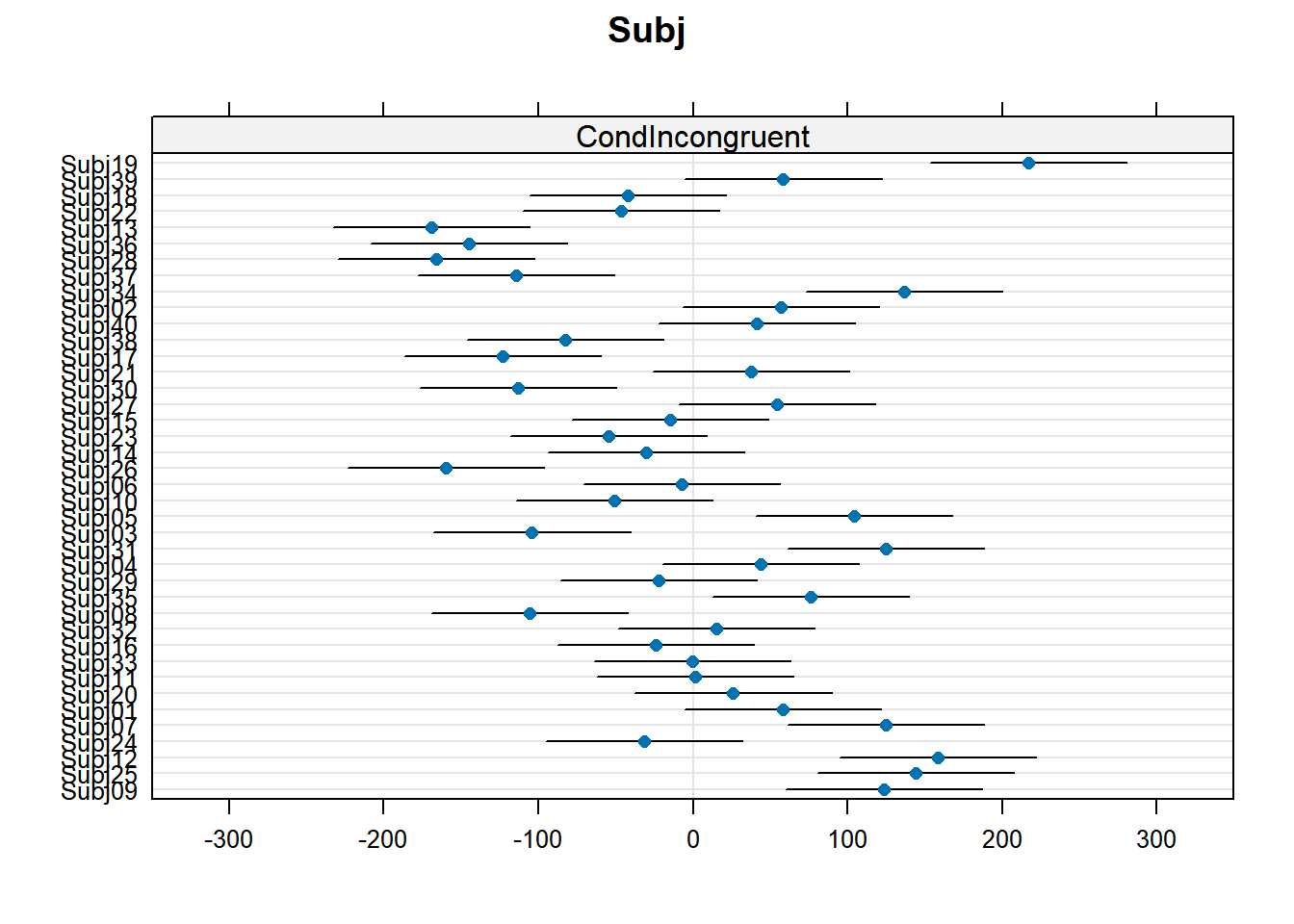
4.3.4.3.2.2 Subject by Condition

plot_model(xmdl.Optimal, type="pred", terms=c("Cond", "Subj"), pred.type="re", ci.lvl = NA, dodge = 0, colors = paletteer_c("grDevices::rainbow", length(unique(dataCong$Subj)))) + theme_bw() + geom_line()

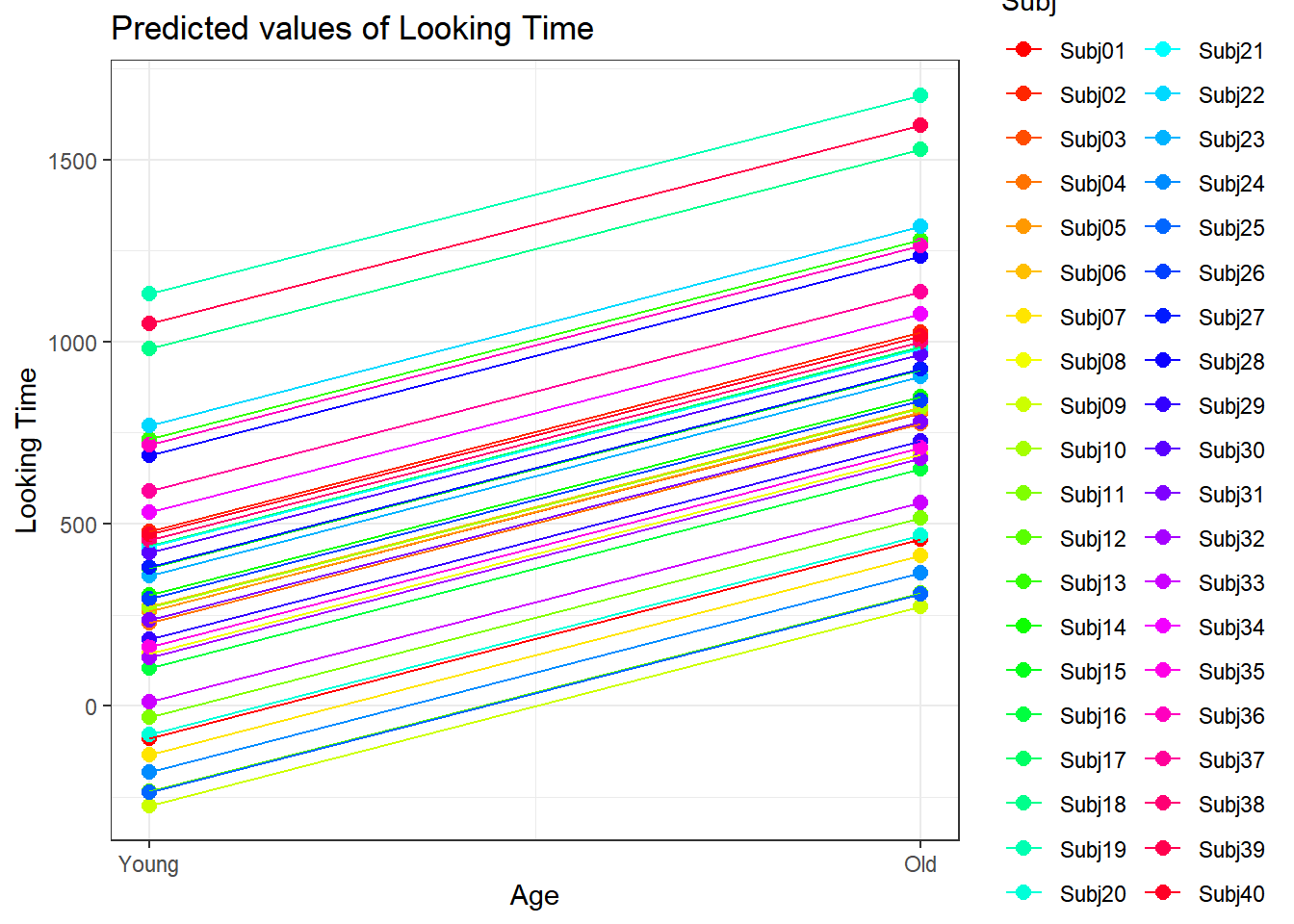
4.3.4.3.2.3 Subject by Age

plot_model(xmdl.Optimal, type="pred", terms=c("Age", "Subj"), pred.type="re", ci.lvl = NA, dodge = 0, colors = paletteer_c("grDevices::rainbow", length(unique(dataCong$Subj)))) + theme_bw() + geom_line()

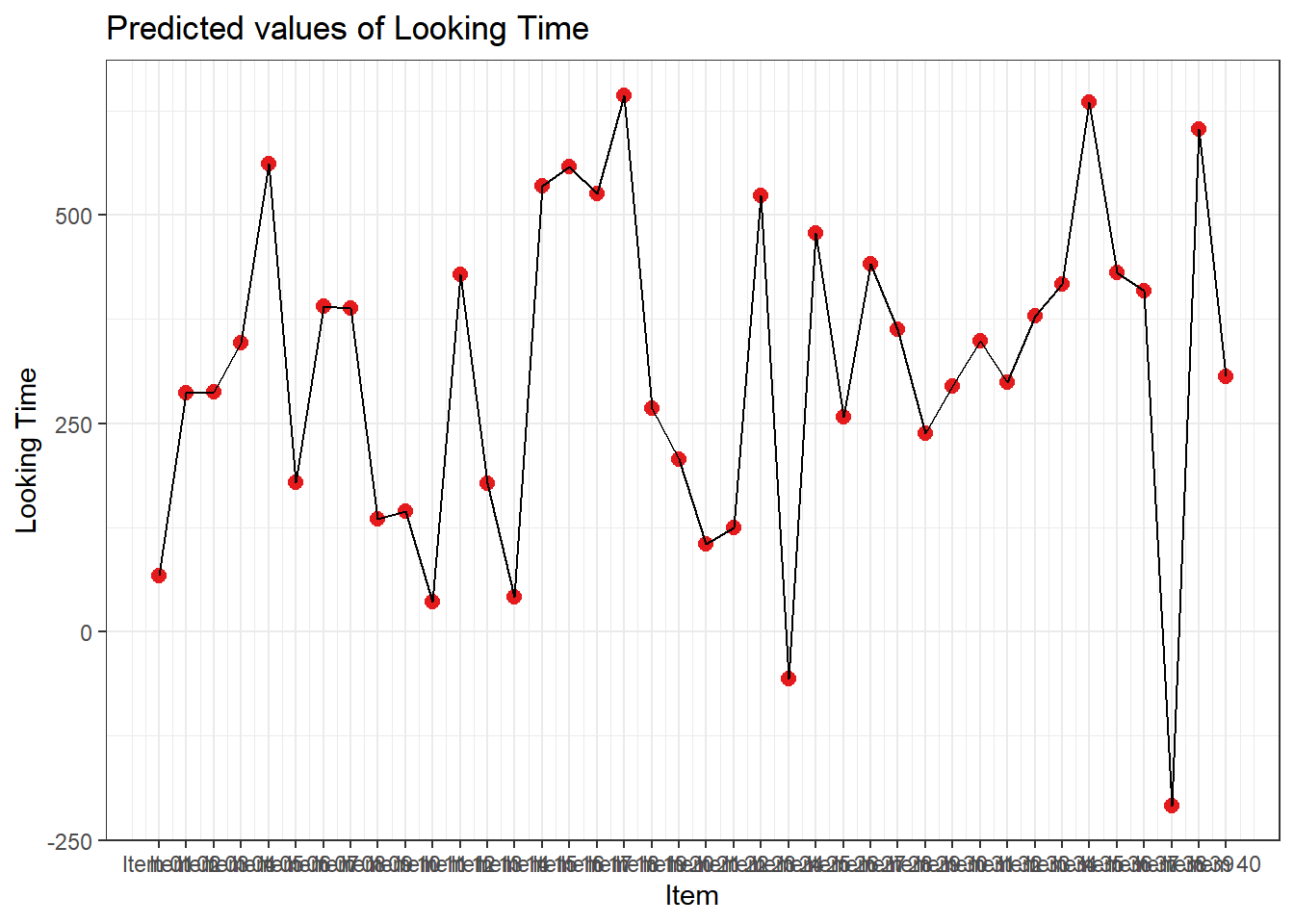
4.3.4.3.2.4 Item

plot_model(xmdl.Optimal, type="pred", terms=c("Item"), pred.type="re", ci.lvl = NA, dodge = 0) + theme_bw() + geom_line()

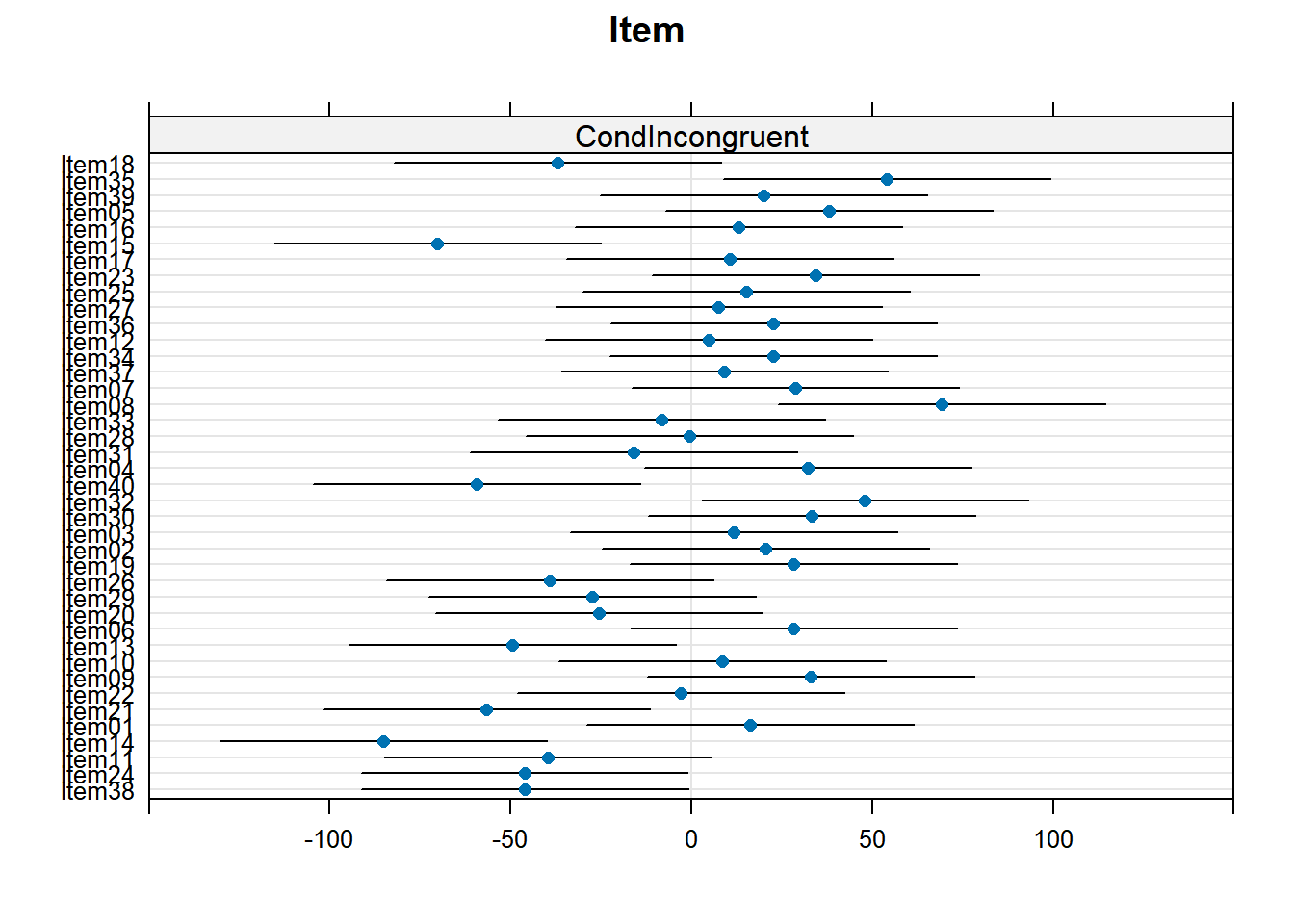
4.3.4.3.2.5 Item by Cond

plot_model(xmdl.Optimal, type="pred", terms=c("Cond", "Item"), pred.type="re", ci.lvl = NA, dodge = 0, colors = paletteer_c("grDevices::rainbow", length(unique(dataCong$Item)))) + theme_bw() + geom_line()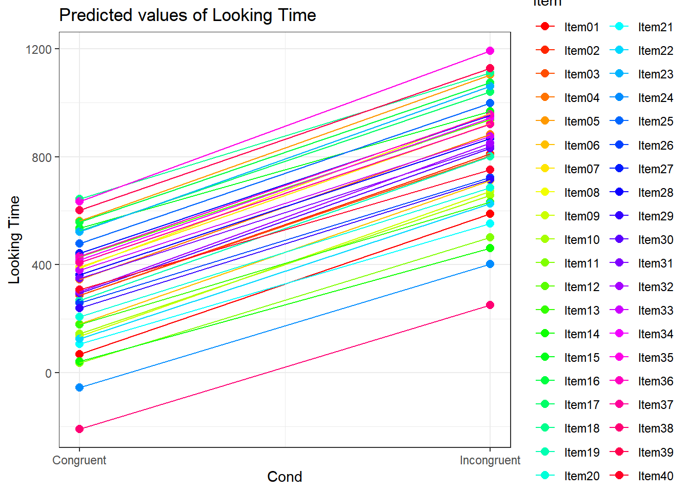

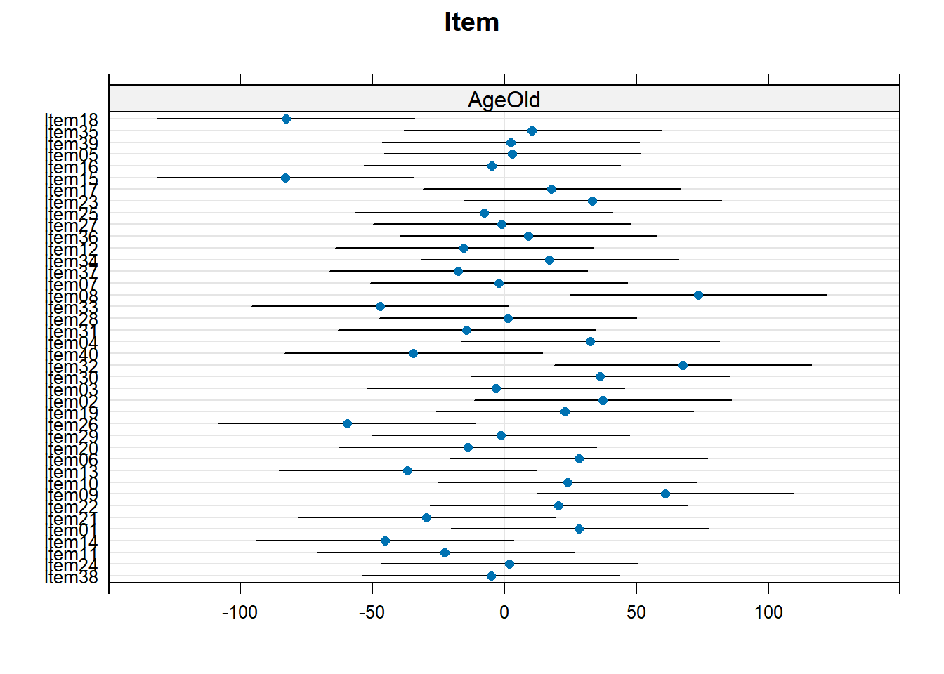
4.3.4.3.2.6 Item by Age

plot_model(xmdl.Optimal, type="pred", terms=c("Age", "Item"), pred.type="re", ci.lvl = NA, dodge = 0, colors = paletteer_c("grDevices::rainbow", length(unique(dataCong$Item)))) + theme_bw() + geom_line()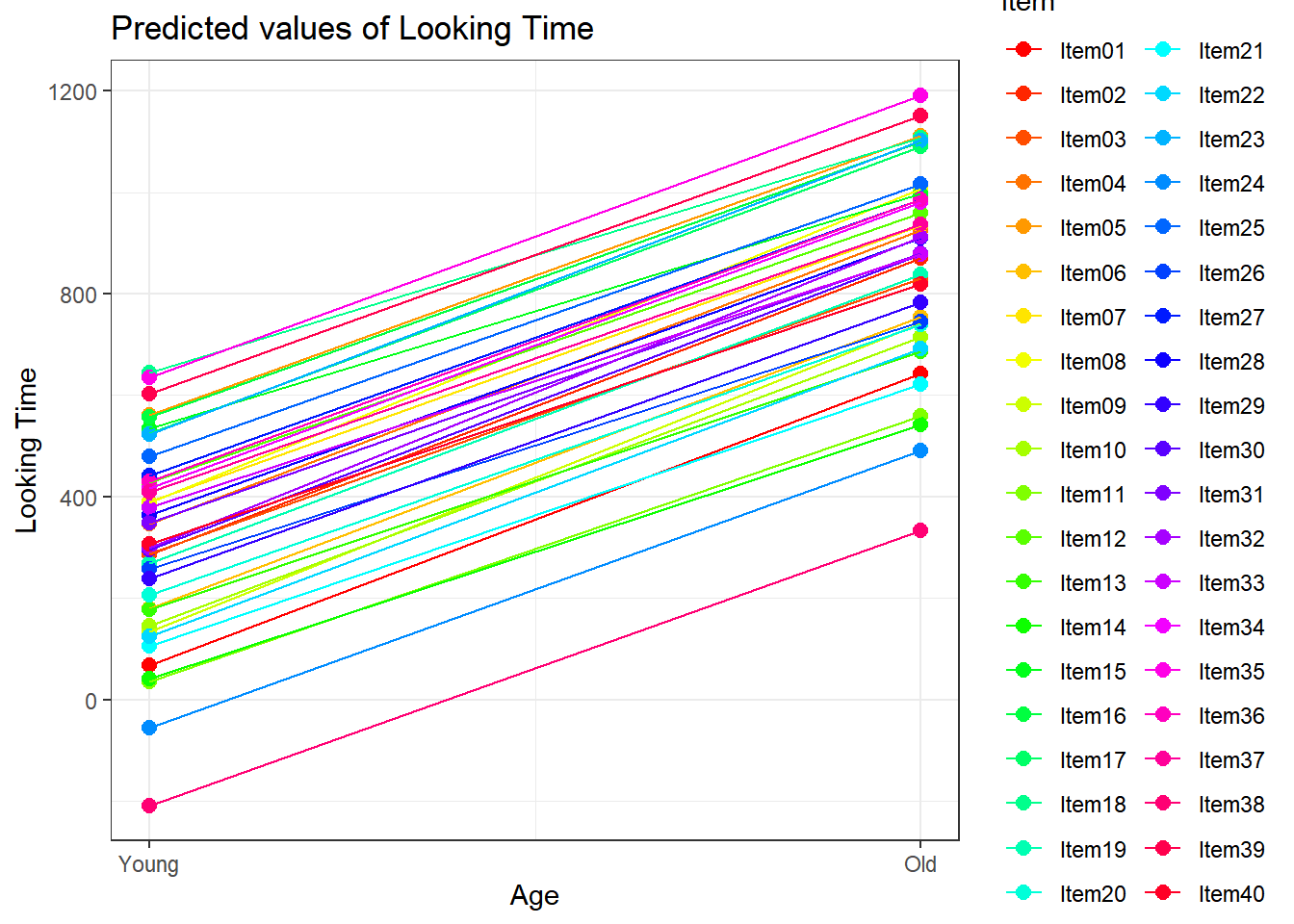

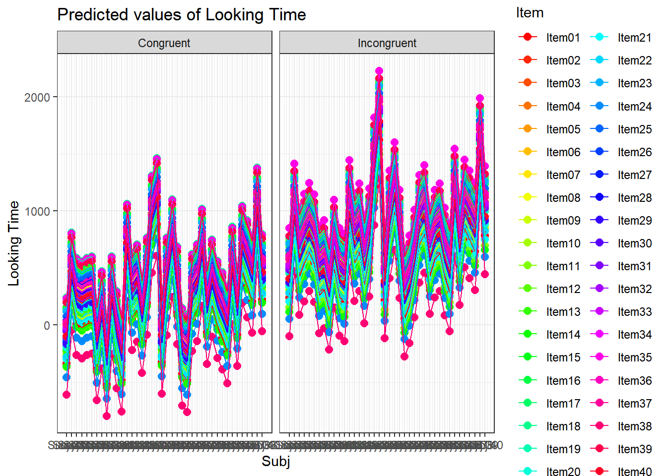
4.3.4.3.2.7 Item by Cond facetted by Age

plot_model(xmdl.Optimal, type="pred", terms=c("Cond", "Item", "Age"), pred.type="re", ci.lvl = NA, dodge = 0, colors = paletteer_c("grDevices::rainbow", length(unique(dataCong$Item)))) + theme_bw() + geom_line()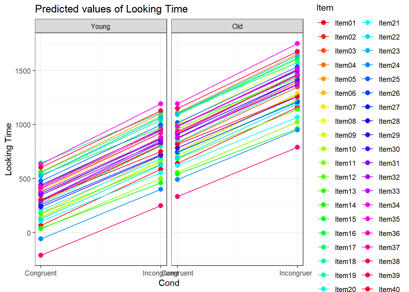

4.3.4.3.2.8 Subject by Item

plot_model(xmdl.Optimal, type="pred", terms=c("Subj", "Item"), pred.type="re", ci.lvl = NA, dodge = 0, colors = paletteer_c("grDevices::rainbow", length(unique(dataCong$Subj)))) + theme_bw() + geom_line()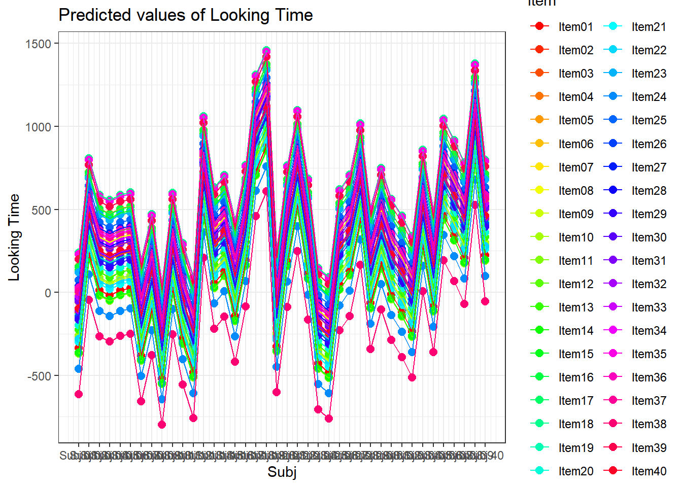

4.3.4.3.2.9 Subject by Item facetted by Cond

plot_model(xmdl.Optimal, type="pred", terms=c("Subj", "Item", "Cond"), pred.type="re", ci.lvl = NA, dodge = 0, colors = paletteer_c("grDevices::rainbow", length(unique(dataCong$Subj)))) + theme_bw() + geom_line()

4.3.4.3.2.10 Subject by Item facetted by Age

plot_model(xmdl.Optimal, type="pred", terms=c("Subj", "Item", "Age"), pred.type="re", ci.lvl = NA, dodge = 0, colors = paletteer_c("grDevices::rainbow", length(unique(dataCong$Subj)))) + theme_bw() + geom_line()

4.3.4.3.3 With `Lattice`

4.3.4.3.3.1 Subject Intercepts

dotplot(ranef(xmdl.Optimal))$Subj[1]

4.3.4.3.3.2 Subject Slopes

dotplot(ranef(xmdl.Optimal), xlim = c(-350, 350))$Subj[2]

4.3.4.3.3.3 Item Intercepts

dotplot(ranef(xmdl.Optimal))$Item[1]

4.3.4.3.3.4 Item Slopes for Cond

dotplot(ranef(xmdl.Optimal), xlim = c(-150, 150))$Item[2]

4.3.4.3.3.5 Item Slopes for Age

dotplot(ranef(xmdl.Optimal), xlim = c(-150, 150))$Item[3]

I hope this tutorial helped you to uncover the role of participants and items and what they can tell us beyond the fixed effect!

4.3.5 Conclusion

In this simulated dataset, we showed how to use Linear Mixed-effects Models, and used a specific approach, named “maximal specification model”. This maximal specification model uses both random intercepts and random slopes. Usually, on any dataset, you are required to formally assess the need for Random slopes.

As a rule of thumb: Any within-subject (or within-item) should be tested for a potential inclusion as a random slope.

Fixed effects provide averages over all observations, even when using mixed effects regressions; we need to explore what random effects (intercepts and slopes) tell us.

In this example, we see that many subjects vary beyond the fixed effect; Standard Errors are not enough to quantify this type of variation. The same is true for items that are not explored routinely!

The approach above used a maximal specification model. This of course depends on the dataset you are working on and requires formal testing. See the package RePsychLing that is on github. The function RePCA is part of the package lme4. You can use it to verify if the model structure is appropriate. However, lme4 will give you directly a warning “is singular” that you can interpret as “over specified model”.