10.4 GLM as a classification tool

10.4.1 Model specification

Let’s run a first GLM (Generalised Linear Model). A GLM uses a special family “binomial” as it assumes the outcome has a binomial distribution. In general, results from a Logistic Regression are close to what we get from SDT.

We will use the same dataset that comes from phonetic research. This dataset is from my current work on the phonetic basis of the guttural natural class in Levantine Arabic. Acoustic analyses were conducted on multiple portions of the VCV sequence, and we report here the averaged results on the first half of V2. Acoustic metrics were obtained via VoiceSauce: various acoustic metrics of supralaryngeal (bark difference) and laryngeal (voice quality via amplitude harmonic differences, noise, energy) were obtained. A total of 23 different acoustic metrics were obtained from 10 participants. Here, we use the data from the first two participants for demonstration purposes (one male and one female). The grouping factor of interest is context with two levels: guttural vs non-guttural. Gutturals include uvular, pharyngealised and pharyngeal consonants; non-gutturals include coronal plain, velar and glottal consonants.

The aim of the study was to evaluate whether the combination of the acoustic metrics provides support for a difference between the two classes of gutturals vs non-gutturals.

We run a GLM with context as our outcome, and Z2-Z1 as our predictor. We want to evaluate whether the two classes can be separated when using the acoustic metric Z2-Z1. Context has two levels, and this will be considered as a binomial distribution.

mdl.glm.Z2mnZ1 <- dfPharV2 %>% 
  glm(context ~ Z2mnZ1, data = ., family = binomial)
summary(mdl.glm.Z2mnZ1)

## 
## Call:
## glm(formula = context ~ Z2mnZ1, family = binomial, data = .)
## 
## Coefficients:
##             Estimate Std. Error z value Pr(>|z|)    
## (Intercept)  0.50112    0.23036   2.175 0.029605 *  
## Z2mnZ1      -0.12281    0.03621  -3.391 0.000696 ***
## ---
## Signif. codes:  0 '***' 0.001 '**' 0.01 '*' 0.05 '.' 0.1 ' ' 1
## 
## (Dispersion parameter for binomial family taken to be 1)
## 
##     Null deviance: 552.89  on 401  degrees of freedom
## Residual deviance: 541.01  on 400  degrees of freedom
## AIC: 545.01
## 
## Number of Fisher Scoring iterations: 4

tidy(mdl.glm.Z2mnZ1) %>% 
  select(term, estimate) %>% 
  mutate(estimate = round(estimate, 3))

## # A tibble: 2 × 2
##   term        estimate
##   <chr>          <dbl>
## 1 (Intercept)    0.501
## 2 Z2mnZ1        -0.123

## to only get the coefficients
mycoef2 <- tidy(mdl.glm.Z2mnZ1) %>% pull(estimate)

10.4.2 Plogis

The result above shows that when moving from the non-guttural (intercept), a unit increase (i.e., guttural) yields a statistically significant decrease in the logodds associated with Z2-Z1. We can evaluate this further from a classification point of view, using plogis.

## non-guttural
plogis(mycoef2[1])

## [1] 0.622722

#guttural
plogis(mycoef2[1] + mycoef2[2])

## [1] 0.5934644

The plogis function provides the probability of being in the guttural class. The intercept (non-guttural) is 0.5, and the guttural class is 0.41. This means that the model predicts that a unit increase in Z2-Z1 yields a decrease of 9% in the probability of being in the guttural class. This is a small effect, but it is statistically significant. The model also provides the logodds associated with the predictor. The logodds are the natural logarithm of the odds ratio, which is the ratio of the probability of being in one class over the other. The logodds are not easy to interpret, but they can be used to evaluate the effect of the predictor on the outcome. The logodds for Z2-Z1 is -0.1, which means that a unit increase in Z2-Z1 yields a decrease of 10% in the odds of being in the guttural class. This is a small effect, but it is statistically significant.

This shows that Z2-Z1 is able to explain the difference in the guttural class with an accuracy of 59%. Let’s continue with this model further.

10.4.3 Model predictions

As above, we obtain predictions from the model. Because we are using a numeric predictor, we need to assign a threshold for the predict function. The threshold can be thought of as telling the predict function to assign any predictions lower than 50% to one group, and any higher to another.

pred.glm.Z2mnZ1 <- predict(mdl.glm.Z2mnZ1, type = "response")>0.5

tbl.glm.Z2mnZ1 <- table(pred.glm.Z2mnZ1, dfPharV2$context)
rownames(tbl.glm.Z2mnZ1) <- c("Non-Guttural", "Guttural")
tbl.glm.Z2mnZ1

##                
## pred.glm.Z2mnZ1 Non-Guttural Guttural
##    Non-Guttural          167       75
##    Guttural               55      105

## from PresenceAbsence
PresenceAbsence::pcc(tbl.glm.Z2mnZ1)

##         PCC    PCC.sd
## 1 0.6766169 0.0233592

PresenceAbsence::specificity(tbl.glm.Z2mnZ1)

##   specificity specificity.sd
## 1   0.5833333     0.03684905

PresenceAbsence::sensitivity(tbl.glm.Z2mnZ1)

##   sensitivity sensitivity.sd
## 1   0.7522523     0.02903959

roc.glm.Z2mnZ1 <- pROC::roc(dfPharV2$context, as.numeric(pred.glm.Z2mnZ1))

## Setting levels: control = Non-Guttural, case = Guttural

## Setting direction: controls < cases

roc.glm.Z2mnZ1

## 
## Call:
## roc.default(response = dfPharV2$context, predictor = as.numeric(pred.glm.Z2mnZ1))
## 
## Data: as.numeric(pred.glm.Z2mnZ1) in 222 controls (dfPharV2$context Non-Guttural) < 180 cases (dfPharV2$context Guttural).
## Area under the curve: 0.6678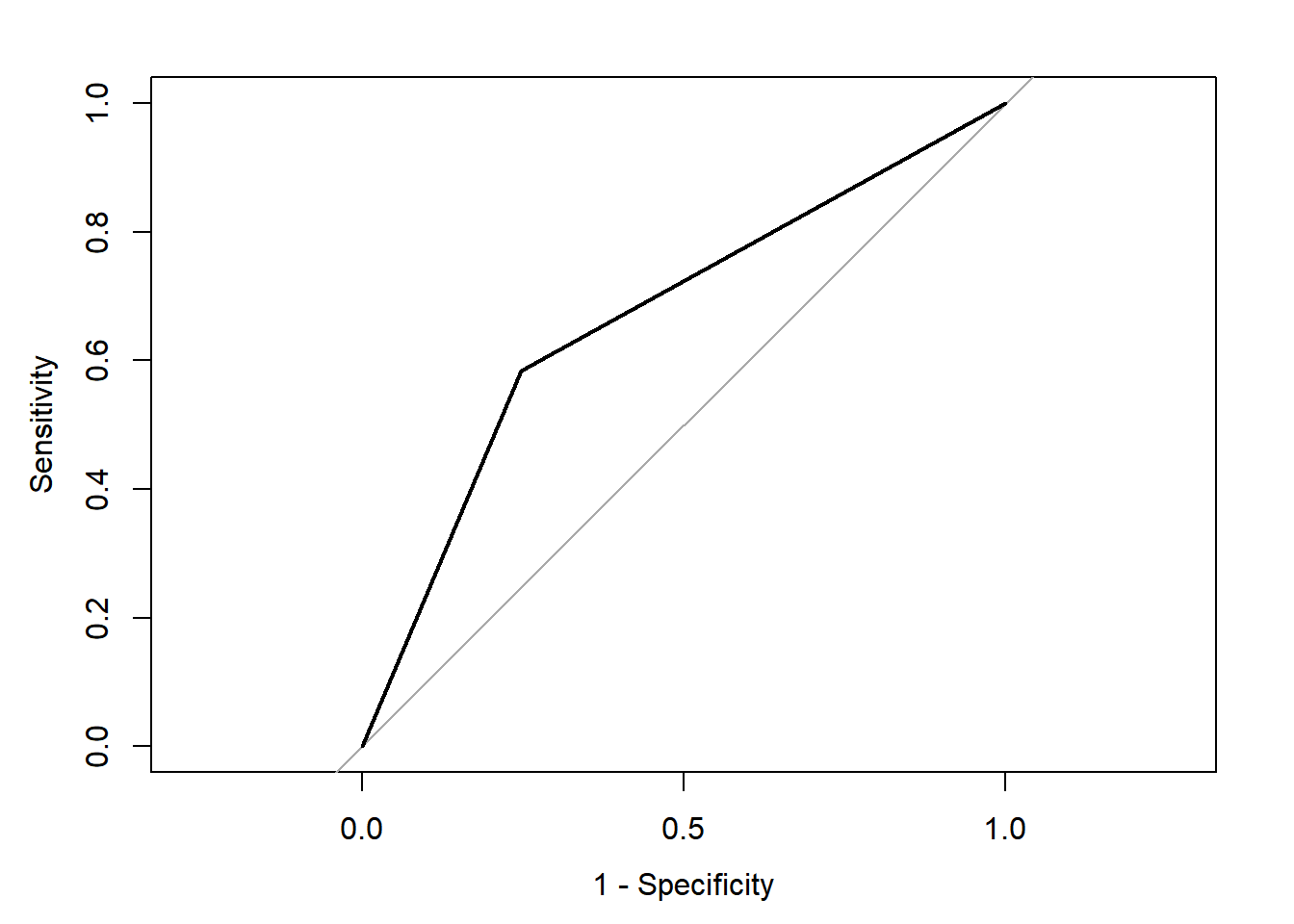

pROC::plot.roc(roc.glm.Z2mnZ1, legacy.axes = TRUE)

The model above was able to explain the difference between the two classes with an accuracy of 67.7%. It has a slightly low specificity (0.583) to detect gutturals, but a sightly high sensitivity (0.752) to reject the non-gutturals. Looking at the confusion matrix, we observe that both groups were relatively accurately identified, but we have relatively large errors (or confusions). The AUC is at 0.6678 which is not too high.

Let’s continue with GLM to evaluate it further. We start by running a correlation test to evaluate issues with GLM.