3.2 Correlation tests

3.2.1 Basic correlations

Let us start with a basic correlation test. We want to evaluate if two numeric variables are correlated with each other.

We use the function cor to obtain the pearson correlation and cor.test to run a basic correlation test on our data with significance testing

cor(english$RTlexdec, english$RTnaming, method = "pearson")

## [1] 0.7587033

cor.test(english$RTlexdec, english$RTnaming)

## 
##  Pearson's product-moment correlation
## 
## data:  english$RTlexdec and english$RTnaming
## t = 78.699, df = 4566, p-value < 2.2e-16
## alternative hypothesis: true correlation is not equal to 0
## 95 percent confidence interval:
##  0.7461195 0.7707453
## sample estimates:
##       cor 
## 0.7587033

What these results are telling us? There is a positive correlation between RTlexdec and RTnaming. The correlation coefficient (R²) is 0.76 (limits between -1 and 1). This correlation is statistically significant with a t value of 78.699, degrees of freedom of 4566 and a p-value < 2.2e-16.

What are the degrees of freedom? These relate to number of total observations - number of comparisons. Here we have 4568 observations in the dataset, and two comparisons, hence 4568 - 2 = 4566.

For the p value, there is a threshold we usually use. This threshold is p = 0.05. This threshold means we have a minimum to consider any difference as significant or not. 0.05 means that we have a probability to find a significant difference that is at 5% or lower. IN our case, the p value is lower that 2.2e-16. How to interpret this number? this tells us to add 15 0s before the 2!! i.e., 0.0000000000000002. This probability is very (very!!) low. So we conclude that there is a statistically significant correlation between the two variables.

The formula to calculate the t value is below.

x̄ = sample mean μ0 = population mean s = sample standard deviation n = sample size

The p value is influenced by various factors, number of observations, strength of the difference, mean values, etc.. You should always be careful with interpreting p values taking everything else into account.

3.2.2 Using the package corrplot

Above, we did a correlation test on two predictors. What if we want to obtain a nice plot of all numeric predictors and add significance levels?

3.2.2.1 Correlation plots

corr <- 
  english %>% 
  select(where(is.numeric)) %>% 
  cor()
corrplot(corr, method = 'ellipse', type = 'upper')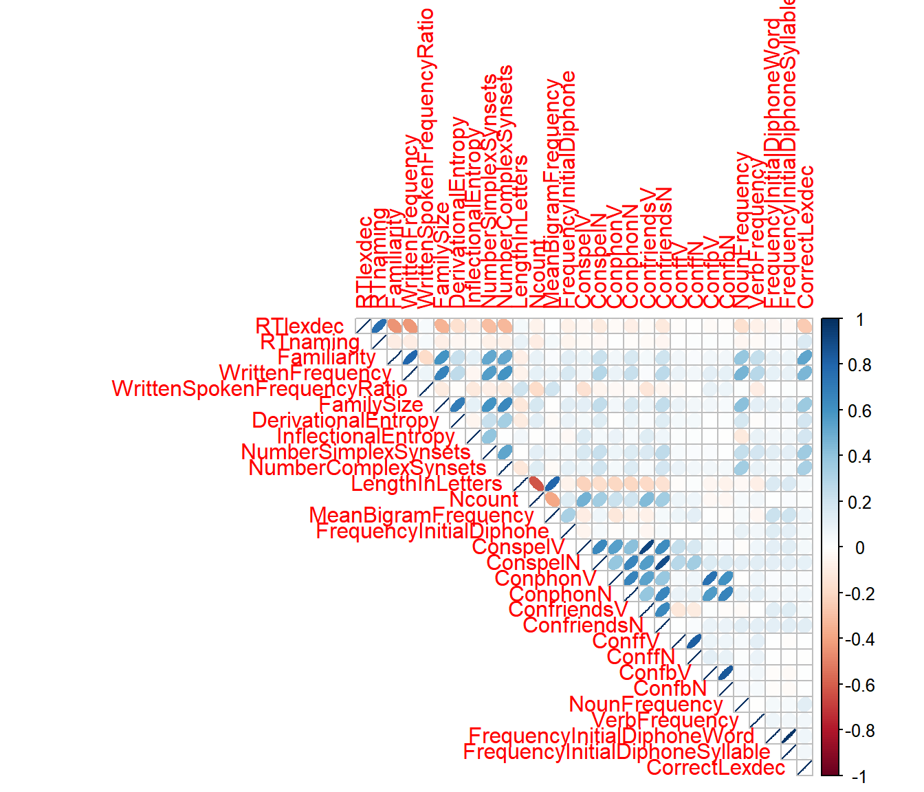

3.2.2.2 More advanced

Let’s first compute the correlations between all numeric variables and plot these with the p values

## correlation using "corrplot"
## based on the function `rcorr' from the `Hmisc` package
## Need to change dataframe into a matrix
corr <- 
  english %>% 
  select(where(is.numeric)) %>% 
  data.matrix(english) %>% 
  rcorr(type = "pearson")
# use corrplot to obtain a nice correlation plot!
corrplot(corr$r, p.mat = corr$P,
         addCoef.col = "black", diag = FALSE, type = "upper", tl.srt = 55)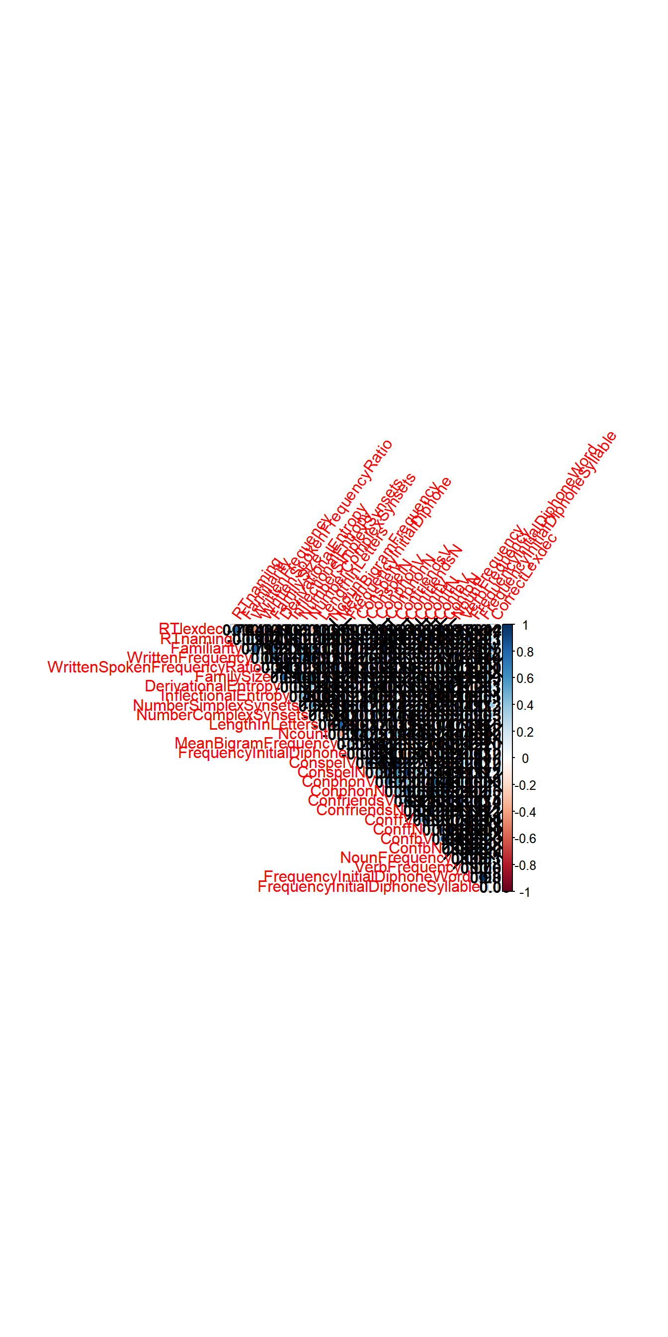

english %>% 
  group_by(AgeSubject) %>% 
  summarise(mean = mean(RTlexdec),
            sd = sd(RTlexdec))

## # A tibble: 2 × 3
##   AgeSubject  mean    sd
##   <fct>      <dbl> <dbl>
## 1 old         6.66 0.116
## 2 young       6.44 0.106