10.5 Issues with GLM (and regression analyses in general)

10.5.1 Correlation tests

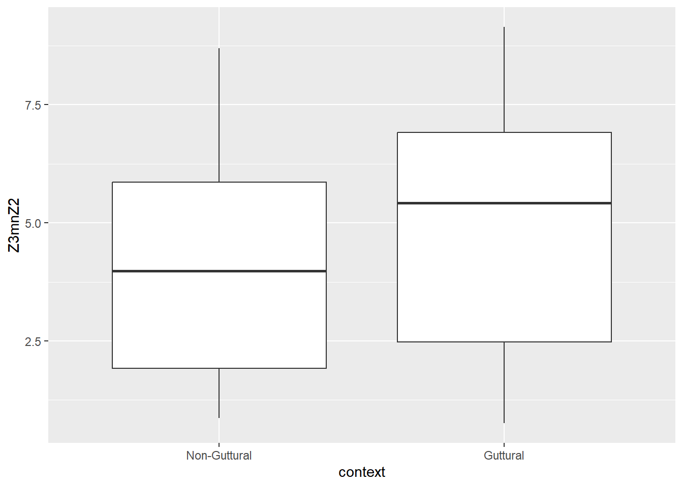
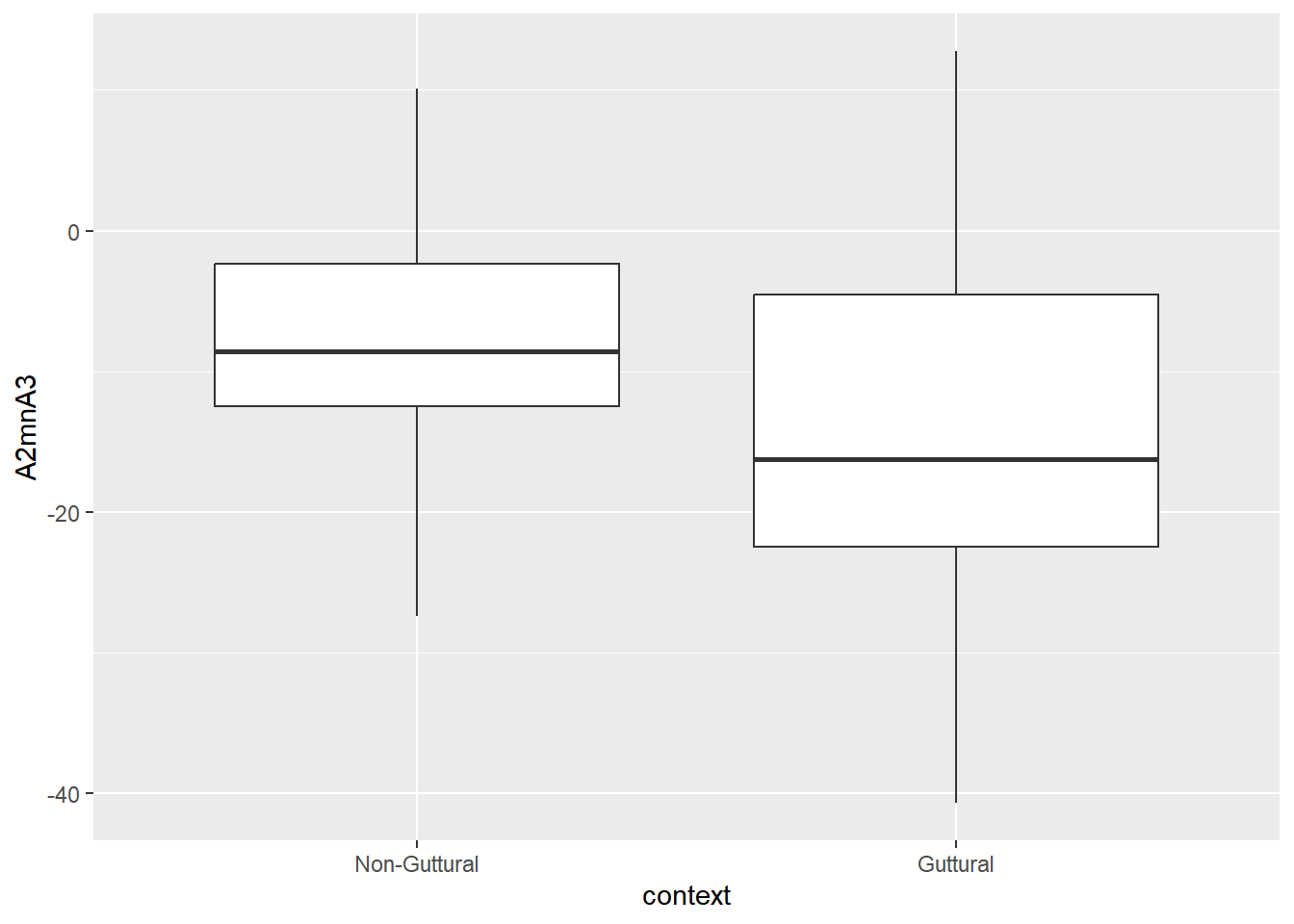
Below, we look at two predictors that are correlated with each other: Z3-Z2 (F3-F2 in Bark) and A2*-A3* (normalised amplitude differences between harmonics closest to F2 and F3). The results of the correlation test shows the two predictors to negatively correlate with each other at a rate of -0.87.

cor.test(dfPharV2$Z3mnZ2, dfPharV2$A2mnA3)

## 
##  Pearson's product-moment correlation
## 
## data:  dfPharV2$Z3mnZ2 and dfPharV2$A2mnA3
## t = -35.864, df = 400, p-value < 2.2e-16
## alternative hypothesis: true correlation is not equal to 0
## 95 percent confidence interval:
##  -0.8947506 -0.8480066
## sample estimates:
##        cor 
## -0.8733751

10.5.2 Plots to visualise the data

dfPharV2 %>% 
  ggplot(aes(x = context, y = Z3mnZ2)) + 
  geom_boxplot()

dfPharV2 %>% 
  ggplot(aes(x = context, y = A2mnA3)) + 
  geom_boxplot()  

As we see from the plot, Z3-Z2 is higher in the guttural, whereas A2*-A3* is lower.

10.5.3 GLM on correlated data

Let’s run a logistic regression as a classification tool to predict the context as a function of each predictor separately and then combined.

dfPharV2 %>% glm(context ~ Z3mnZ2, data = ., family = binomial) %>% summary()

## 
## Call:
## glm(formula = context ~ Z3mnZ2, family = binomial, data = .)
## 
## Coefficients:
##             Estimate Std. Error z value Pr(>|z|)    
## (Intercept) -0.99451    0.23061  -4.313 1.61e-05 ***
## Z3mnZ2       0.17440    0.04553   3.831 0.000128 ***
## ---
## Signif. codes:  0 '***' 0.001 '**' 0.01 '*' 0.05 '.' 0.1 ' ' 1
## 
## (Dispersion parameter for binomial family taken to be 1)
## 
##     Null deviance: 552.89  on 401  degrees of freedom
## Residual deviance: 537.74  on 400  degrees of freedom
## AIC: 541.74
## 
## Number of Fisher Scoring iterations: 4

dfPharV2 %>% glm(context ~ A2mnA3, data = ., family = binomial) %>% summary()

## 
## Call:
## glm(formula = context ~ A2mnA3, family = binomial, data = .)
## 
## Coefficients:
##             Estimate Std. Error z value Pr(>|z|)    
## (Intercept) -0.98961    0.16632  -5.950 2.68e-09 ***
## A2mnA3      -0.06973    0.01122  -6.215 5.12e-10 ***
## ---
## Signif. codes:  0 '***' 0.001 '**' 0.01 '*' 0.05 '.' 0.1 ' ' 1
## 
## (Dispersion parameter for binomial family taken to be 1)
## 
##     Null deviance: 552.89  on 401  degrees of freedom
## Residual deviance: 508.51  on 400  degrees of freedom
## AIC: 512.51
## 
## Number of Fisher Scoring iterations: 4

dfPharV2 %>% glm(context ~ Z3mnZ2 + A2mnA3, data = ., family = binomial) %>% summary()

## 
## Call:
## glm(formula = context ~ Z3mnZ2 + A2mnA3, family = binomial, data = .)
## 
## Coefficients:
##             Estimate Std. Error z value Pr(>|z|)    
## (Intercept) -0.10996    0.27830  -0.395 0.692754    
## Z3mnZ2      -0.39266    0.10201  -3.849 0.000118 ***
## A2mnA3      -0.14930    0.02418  -6.175 6.61e-10 ***
## ---
## Signif. codes:  0 '***' 0.001 '**' 0.01 '*' 0.05 '.' 0.1 ' ' 1
## 
## (Dispersion parameter for binomial family taken to be 1)
## 
##     Null deviance: 552.89  on 401  degrees of freedom
## Residual deviance: 492.50  on 399  degrees of freedom
## AIC: 498.5
## 
## Number of Fisher Scoring iterations: 4

When looking at the three models above, it is clear that the logodd value for Z3-Z2 is positive, whereas it is negative for A2*-A3*. When adding the two predictors together, there is clear suppression: the coefficients for both predictors are now negative. The relatively high correlation between the predictors affected the coefficients and changed the direction of the slope; collinearity is harmful for any regression analysis.

In the following, we introduce decision trees followed by Random Forest as a way to deal with collinearity and to make sense of multivariate predictors.