3.3 Linear Models

Up to now, we have looked at descriptive statistics, and evaluated summaries, correlations in the data (with p values).

We are now interested in looking at group differences.

3.3.1 Introduction

The basic assumption of a Linear model is to create a regression analysis on the data. We have an outcome (or dependent variable) and a predictor (or an independent variable). The formula of a linear model is as follows outcome ~ predictor that can be read as “outcome as a function of the predictor”. We can add “1” to specify an intercept, but this is by default added to the model

3.3.1.1 Model estimation

english2 <- english %>% 
  mutate(AgeSubject = factor(AgeSubject, levels = c("young", "old")))
mdl.lm <- english2 %>% 
  lm(RTlexdec ~ AgeSubject, data = .)
#lm(RTlexdec ~ AgeSubject, data = english)
mdl.lm #also print(mdl.lm)

## 
## Call:
## lm(formula = RTlexdec ~ AgeSubject, data = .)
## 
## Coefficients:
##   (Intercept)  AgeSubjectold  
##        6.4392         0.2217

summary(mdl.lm)

## 
## Call:
## lm(formula = RTlexdec ~ AgeSubject, data = .)
## 
## Residuals:
##      Min       1Q   Median       3Q      Max 
## -0.25776 -0.08339 -0.01669  0.06921  0.52685 
## 
## Coefficients:
##               Estimate Std. Error t value Pr(>|t|)    
## (Intercept)   6.439237   0.002324 2771.03   <2e-16 ***
## AgeSubjectold 0.221721   0.003286   67.47   <2e-16 ***
## ---
## Signif. codes:  0 '***' 0.001 '**' 0.01 '*' 0.05 '.' 0.1 ' ' 1
## 
## Residual standard error: 0.1111 on 4566 degrees of freedom
## Multiple R-squared:  0.4992, Adjusted R-squared:  0.4991 
## F-statistic:  4552 on 1 and 4566 DF,  p-value: < 2.2e-16

3.3.2 Role of coding schemes

3.3.2.1 Intro

There are other coding schemes that can be used. See Schad et al. (2020): “How to capitalize on a priori contrasts in linear (mixed) models: A tutorial”. Journal of Memory and Language,vol. 110, 104038.

We have:

The treatment coding
The contrast or sum coding
The polynomial coding
The Repeated coding
The helmert coding

The first two are the most commonly used coding schemes, but see the paper for why one can use the others.

3.3.2.2 Treatment coding

By default, R uses a treatment coding scheme. By this we mean that the intercept has the outcome of a specific level in the dataset (usually, the first in alphabetical order, unless you have changed that!). In our example above, we changed the reference level of the variable AgeSubject to be “young” vs “old”. What we see as an result in our LM is the intercept (=Young) vs “AgeSubjectold”. This will mean we are looking at the difference between the reference level and all other levels.

The code below allows you to see what the coding scheme is.

english2$AgeSubject2 <- english2$AgeSubject

contrasts(english2$AgeSubject2) <- contr.treatment(2)
contrasts(english2$AgeSubject2)

##       2
## young 0
## old   1

mdl.lm.T <- english2 %>% 
  lm(RTlexdec ~ AgeSubject2, data = .)
#lm(RTlexdec ~ AgeSubject, data = english)
mdl.lm.T #also print(mdl.lm)

## 
## Call:
## lm(formula = RTlexdec ~ AgeSubject2, data = .)
## 
## Coefficients:
##  (Intercept)  AgeSubject22  
##       6.4392        0.2217

summary(mdl.lm.T)

## 
## Call:
## lm(formula = RTlexdec ~ AgeSubject2, data = .)
## 
## Residuals:
##      Min       1Q   Median       3Q      Max 
## -0.25776 -0.08339 -0.01669  0.06921  0.52685 
## 
## Coefficients:
##              Estimate Std. Error t value Pr(>|t|)    
## (Intercept)  6.439237   0.002324 2771.03   <2e-16 ***
## AgeSubject22 0.221721   0.003286   67.47   <2e-16 ***
## ---
## Signif. codes:  0 '***' 0.001 '**' 0.01 '*' 0.05 '.' 0.1 ' ' 1
## 
## Residual standard error: 0.1111 on 4566 degrees of freedom
## Multiple R-squared:  0.4992, Adjusted R-squared:  0.4991 
## F-statistic:  4552 on 1 and 4566 DF,  p-value: < 2.2e-16

3.3.2.3 Contrast (or sum) coding

3.3.2.3.1 Default

Let’s change the coding scheme and see the difference in the output.

english2 <- english2 %>% 
  mutate(AgeSubject2 = factor(AgeSubject2, levels = c("old", "young")))

contrasts(english2$AgeSubject2) <- contr.sum(2)
contrasts(english2$AgeSubject2)

##       [,1]
## old      1
## young   -1

mdl.lm.C <- english2 %>% 
  lm(RTlexdec ~ AgeSubject2, data = .)
#lm(RTlexdec ~ AgeSubject, data = english)
mdl.lm.C #also print(mdl.lm)

## 
## Call:
## lm(formula = RTlexdec ~ AgeSubject2, data = .)
## 
## Coefficients:
##  (Intercept)  AgeSubject21  
##       6.5501        0.1109

summary(mdl.lm.C)

## 
## Call:
## lm(formula = RTlexdec ~ AgeSubject2, data = .)
## 
## Residuals:
##      Min       1Q   Median       3Q      Max 
## -0.25776 -0.08339 -0.01669  0.06921  0.52685 
## 
## Coefficients:
##              Estimate Std. Error t value Pr(>|t|)    
## (Intercept)  6.550097   0.001643 3986.29   <2e-16 ***
## AgeSubject21 0.110861   0.001643   67.47   <2e-16 ***
## ---
## Signif. codes:  0 '***' 0.001 '**' 0.01 '*' 0.05 '.' 0.1 ' ' 1
## 
## Residual standard error: 0.1111 on 4566 degrees of freedom
## Multiple R-squared:  0.4992, Adjusted R-squared:  0.4991 
## F-statistic:  4552 on 1 and 4566 DF,  p-value: < 2.2e-16

With contrast (or sum) coding, the intercept is almost the same as before (treatment = 6.439237 vs contrast = 6.550097). The intercept is now the average of all of the data points

english2 %>% 
  mutate(meanRTlexdec = mean(RTlexdec)) %>% 
  select(meanRTlexdec) %>%
  head(10)

##    meanRTlexdec
## 1      6.550097
## 2      6.550097
## 3      6.550097
## 4      6.550097
## 5      6.550097
## 6      6.550097
## 7      6.550097
## 8      6.550097
## 9      6.550097
## 10     6.550097

The coefficient for “old” is different. It is now nearly half of that in the treatment coding (0.221721 vs 0.110861). Why is this the case? In treatment coding, the distance between old and young was of 1 (1- 0 = 1), in contrast coding, it is of 2 (1 - -1 = 2). The coefficient of the intercept is exactly the same; for the second, it is half of the one above (0.221721 / 1 = 0.221721; 0.221721 / 2 = 0.110861)!

How to interpret the coefficient for the level “old”? It is the distance from the average!

Let’s change slightly the coding scheme

3.3.2.3.2 Modified

english2 <- english2 %>% 
  mutate(AgeSubject2 = factor(AgeSubject, levels = c("young", "old")))

contrasts(english2$AgeSubject2) <- c(-0.5, 0.5)
contrasts(english2$AgeSubject2)

##       [,1]
## young -0.5
## old    0.5

mdl.lmC.2 <- english2 %>% 
  lm(RTlexdec ~ AgeSubject2, data = .)
#lm(RTlexdec ~ AgeSubject, data = english)
mdl.lmC.2 #also print(mdl.lmC.2)

## 
## Call:
## lm(formula = RTlexdec ~ AgeSubject2, data = .)
## 
## Coefficients:
##  (Intercept)  AgeSubject21  
##       6.5501        0.2217

summary(mdl.lmC.2)

## 
## Call:
## lm(formula = RTlexdec ~ AgeSubject2, data = .)
## 
## Residuals:
##      Min       1Q   Median       3Q      Max 
## -0.25776 -0.08339 -0.01669  0.06921  0.52685 
## 
## Coefficients:
##              Estimate Std. Error t value Pr(>|t|)    
## (Intercept)  6.550097   0.001643 3986.29   <2e-16 ***
## AgeSubject21 0.221721   0.003286   67.47   <2e-16 ***
## ---
## Signif. codes:  0 '***' 0.001 '**' 0.01 '*' 0.05 '.' 0.1 ' ' 1
## 
## Residual standard error: 0.1111 on 4566 degrees of freedom
## Multiple R-squared:  0.4992, Adjusted R-squared:  0.4991 
## F-statistic:  4552 on 1 and 4566 DF,  p-value: < 2.2e-16

Our intercept is still the average of all datapoints of the dependent variable; that of “old” is now at 0.221721 as expected. The distance between young and old is of 1 (0.5 - -0.5 = 1).

When and why do we use the different coding schemes? We use it to make the intercept more interpretable. This is especially the case when having more than two categorical predictors, or interactions between a numeric and a categorical predictor. Read the paper and the Bodo Winter’s book for more details.

3.3.3 Further steps

3.3.3.1 Tidying the output

We use our original model with treatment coding.

# from library(broom)
tidy(mdl.lm) %>% 
  select(term, estimate) %>% 
  mutate(estimate = round(estimate, 3))

## # A tibble: 2 × 2
##   term          estimate
##   <chr>            <dbl>
## 1 (Intercept)      6.44 
## 2 AgeSubjectold    0.222

mycoefE <- tidy(mdl.lm) %>% pull(estimate)

Obtaining mean values from our model

#old
mycoefE[1]

## [1] 6.439237

#young
mycoefE[1] + mycoefE[2]

## [1] 6.660958

3.3.3.2 Nice table of our model summary

We can also obtain a nice table of our model summary. We can use the package knitr or xtable

3.3.3.2.1 Directly from model summary

kable(summary(mdl.lm)$coef, digits = 3)

	Estimate	Std. Error	t value	Pr(>\|t\|)
(Intercept)	6.439	0.002	2771.027	0
AgeSubjectold	0.222	0.003	67.468	0

3.3.3.2.2 From the `tidy` output

mdl.lmT <- tidy(mdl.lm)
kable(mdl.lmT, digits = 3)

term	estimate	std.error	statistic	p.value
(Intercept)	6.439	0.002	2771.027	0
AgeSubjectold	0.222	0.003	67.468	0

3.3.3.2.3 Model’s fit

print(tab_model(mdl.lm, file = paste0("outputs/mdl_lm.html")))
htmltools::includeHTML("outputs/mdl_lm.html")

	R Tlexdec
Predictors	Estimates	CI	p
(Intercept)	6.44	6.43 – 6.44	<0.001
AgeSubject [old]	0.22	0.22 – 0.23	<0.001
Observations	4568
R² / R² adjusted	0.499 / 0.499

3.3.3.3 Dissecting the model

Let us dissect the model. If you use “str”, you will be able to see what is available under our linear model. To access some info from the model

3.3.3.3.1 “str” and “coef”

str(mdl.lm)

## List of 13
##  $ coefficients : Named num [1:2] 6.439 0.222
##   ..- attr(*, "names")= chr [1:2] "(Intercept)" "AgeSubjectold"
##  $ residuals    : Named num [1:4568] 0.1045 -0.0416 -0.1343 -0.015 0.0114 ...
##   ..- attr(*, "names")= chr [1:4568] "1" "2" "3" "4" ...
##  $ effects      : Named num [1:4568] -442.7013 7.4927 -0.1352 -0.0159 0.0105 ...
##   ..- attr(*, "names")= chr [1:4568] "(Intercept)" "AgeSubjectold" "" "" ...
##  $ rank         : int 2
##  $ fitted.values: Named num [1:4568] 6.44 6.44 6.44 6.44 6.44 ...
##   ..- attr(*, "names")= chr [1:4568] "1" "2" "3" "4" ...
##  $ assign       : int [1:2] 0 1
##  $ qr           :List of 5
##   ..$ qr   : num [1:4568, 1:2] -67.587 0.0148 0.0148 0.0148 0.0148 ...
##   .. ..- attr(*, "dimnames")=List of 2
##   .. .. ..$ : chr [1:4568] "1" "2" "3" "4" ...
##   .. .. ..$ : chr [1:2] "(Intercept)" "AgeSubjectold"
##   .. ..- attr(*, "assign")= int [1:2] 0 1
##   .. ..- attr(*, "contrasts")=List of 1
##   .. .. ..$ AgeSubject: chr "contr.treatment"
##   ..$ qraux: num [1:2] 1.01 1.01
##   ..$ pivot: int [1:2] 1 2
##   ..$ tol  : num 1e-07
##   ..$ rank : int 2
##   ..- attr(*, "class")= chr "qr"
##  $ df.residual  : int 4566
##  $ contrasts    :List of 1
##   ..$ AgeSubject: chr "contr.treatment"
##  $ xlevels      :List of 1
##   ..$ AgeSubject: chr [1:2] "young" "old"
##  $ call         : language lm(formula = RTlexdec ~ AgeSubject, data = .)
##  $ terms        :Classes 'terms', 'formula'  language RTlexdec ~ AgeSubject
##   .. ..- attr(*, "variables")= language list(RTlexdec, AgeSubject)
##   .. ..- attr(*, "factors")= int [1:2, 1] 0 1
##   .. .. ..- attr(*, "dimnames")=List of 2
##   .. .. .. ..$ : chr [1:2] "RTlexdec" "AgeSubject"
##   .. .. .. ..$ : chr "AgeSubject"
##   .. ..- attr(*, "term.labels")= chr "AgeSubject"
##   .. ..- attr(*, "order")= int 1
##   .. ..- attr(*, "intercept")= int 1
##   .. ..- attr(*, "response")= int 1
##   .. ..- attr(*, ".Environment")=<environment: 0x00000266f9b6e9d8> 
##   .. ..- attr(*, "predvars")= language list(RTlexdec, AgeSubject)
##   .. ..- attr(*, "dataClasses")= Named chr [1:2] "numeric" "factor"
##   .. .. ..- attr(*, "names")= chr [1:2] "RTlexdec" "AgeSubject"
##  $ model        :'data.frame':   4568 obs. of  2 variables:
##   ..$ RTlexdec  : num [1:4568] 6.54 6.4 6.3 6.42 6.45 ...
##   ..$ AgeSubject: Factor w/ 2 levels "young","old": 1 1 1 1 1 1 1 1 1 1 ...
##   ..- attr(*, "terms")=Classes 'terms', 'formula'  language RTlexdec ~ AgeSubject
##   .. .. ..- attr(*, "variables")= language list(RTlexdec, AgeSubject)
##   .. .. ..- attr(*, "factors")= int [1:2, 1] 0 1
##   .. .. .. ..- attr(*, "dimnames")=List of 2
##   .. .. .. .. ..$ : chr [1:2] "RTlexdec" "AgeSubject"
##   .. .. .. .. ..$ : chr "AgeSubject"
##   .. .. ..- attr(*, "term.labels")= chr "AgeSubject"
##   .. .. ..- attr(*, "order")= int 1
##   .. .. ..- attr(*, "intercept")= int 1
##   .. .. ..- attr(*, "response")= int 1
##   .. .. ..- attr(*, ".Environment")=<environment: 0x00000266f9b6e9d8> 
##   .. .. ..- attr(*, "predvars")= language list(RTlexdec, AgeSubject)
##   .. .. ..- attr(*, "dataClasses")= Named chr [1:2] "numeric" "factor"
##   .. .. .. ..- attr(*, "names")= chr [1:2] "RTlexdec" "AgeSubject"
##  - attr(*, "class")= chr "lm"

coef(mdl.lm)

##   (Intercept) AgeSubjectold 
##     6.4392366     0.2217215

## same as 
## mdl.lm$coefficients

3.3.3.3.2 “coef” and “coefficients”

What if I want to obtain the “Intercept”? Or the coefficient for distance? What if I want the full row for distance?

coef(mdl.lm)[1] # same as mdl.lm$coefficients[1]

## (Intercept) 
##    6.439237

coef(mdl.lm)[2] # same as mdl.lm$coefficients[2]

## AgeSubjectold 
##     0.2217215

summary(mdl.lm)$coefficients[2, ] # full row

##    Estimate  Std. Error     t value    Pr(>|t|) 
##  0.22172146  0.00328631 67.46820211  0.00000000

summary(mdl.lm)$coefficients[2, 4] #for p value

## [1] 0

3.3.3.3.3 Residuals

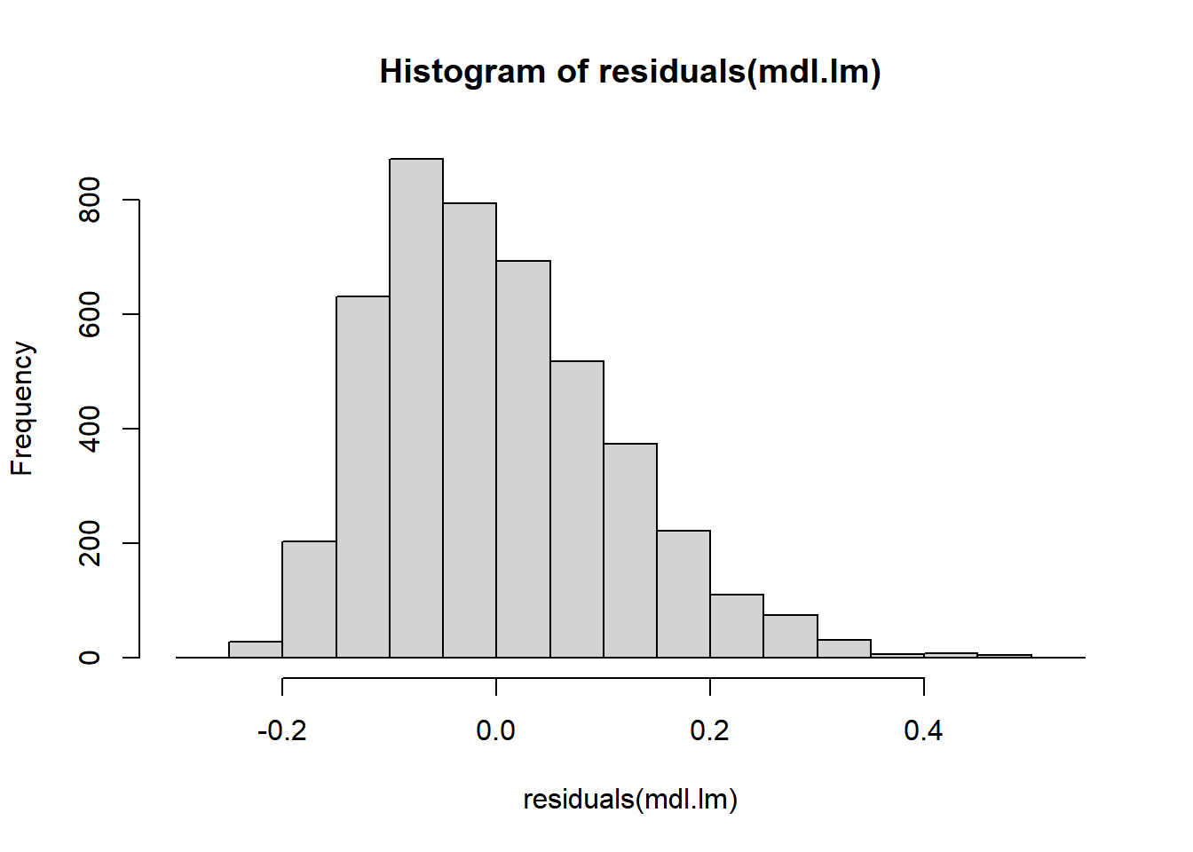
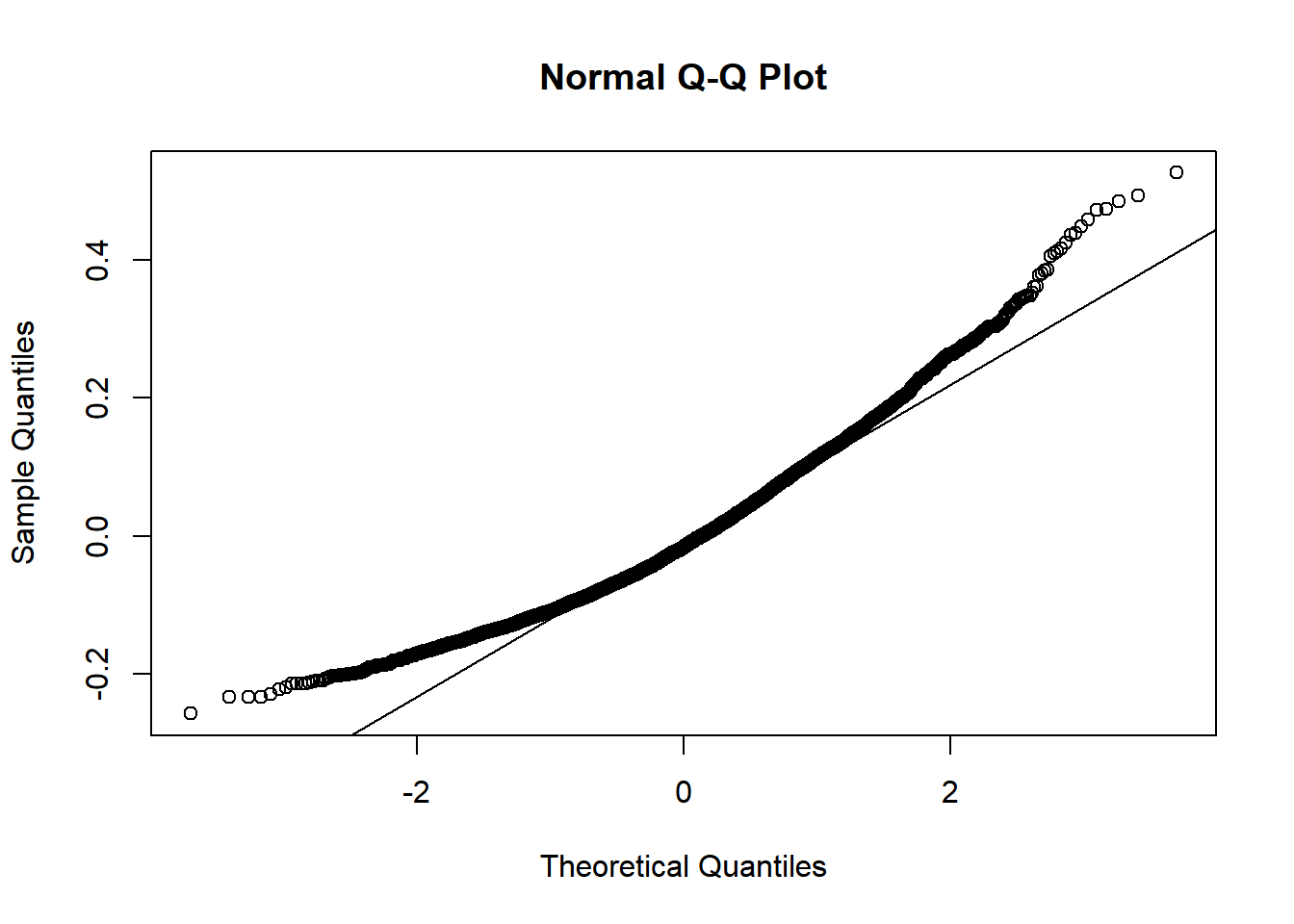
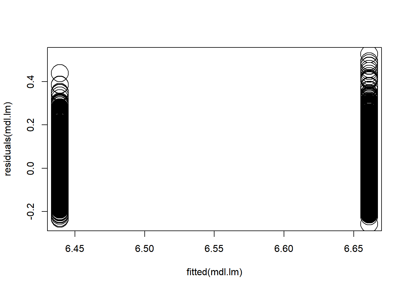
What about residuals (difference between the observed value and the estimated value of the quantity) and fitted values? This allows us to evaluate how normal our residuals are and how different they are from a normal distribution.

3.3.3.3.3.1 Histogram

hist(residuals(mdl.lm))

3.3.3.3.3.2 qqplots

qqnorm(residuals(mdl.lm)); qqline(residuals(mdl.lm))

3.3.3.3.3.3 Residuals vs fitted values

plot(fitted(mdl.lm), residuals(mdl.lm), cex = 4)

3.3.3.3.3.4 Generating and plotting residual plot with `DHARMa`

sim_residuals <- simulateResiduals(mdl.lm)
plot(sim_residuals)

3.3.3.3.4 Goodness of fit?

AIC(mdl.lm) # Akaike's Information Criterion, lower values are better

## [1] -7110.962

BIC(mdl.lm) # Bayesian AIC

## [1] -7091.682

logLik(mdl.lm)  # log likelihood

## 'log Lik.' 3558.481 (df=3)

Or use the following from broom

glance(mdl.lm)

## # A tibble: 1 × 12
##   r.squared adj.r.squared sigma statistic p.value    df logLik    AIC    BIC
##       <dbl>         <dbl> <dbl>     <dbl>   <dbl> <dbl>  <dbl>  <dbl>  <dbl>
## 1     0.499         0.499 0.111     4552.       0     1  3558. -7111. -7092.
## # ℹ 3 more variables: deviance <dbl>, df.residual <int>, nobs <int>

3.3.3.3.5 Significance testing

Are the above informative? of course not directly. If we want to test for overall significance of model. We run a null model (aka intercept only) and compare models.

mdl.lm.Null <- english %>% 
  lm(RTlexdec ~ 1, data = .)
mdl.comp <- anova(mdl.lm.Null, mdl.lm)
mdl.comp

## Analysis of Variance Table
## 
## Model 1: RTlexdec ~ 1
## Model 2: RTlexdec ~ AgeSubject
##   Res.Df     RSS Df Sum of Sq    F    Pr(>F)    
## 1   4567 112.456                                
## 2   4566  56.314  1    56.141 4552 < 2.2e-16 ***
## ---
## Signif. codes:  0 '***' 0.001 '**' 0.01 '*' 0.05 '.' 0.1 ' ' 1

The results show that adding the variable “AgeSubject” improves the model fit. We can write this as follows: Model comparison showed that the addition of AgeSubject improved the model fit when compared with an intercept only model (\(F\)(1) = 4551.96, p < 0) (F(1) = 4552 , p < 2.2e-16)

3.3.4 Plotting fitted values

3.3.4.1 Trend line

Let’s plot our fitted values but only for the trend line

english %>% 
  ggplot(aes(x = AgeSubject, y = RTlexdec))+
  geom_boxplot()+
  theme_bw() + theme(text = element_text(size = 15))+
  geom_smooth(aes(x = as.numeric(AgeSubject), y = predict(mdl.lm)), method = "lm", color = "blue") + 
  labs(x = "Age", y = "RTLexDec", title = "Boxplot and predicted trend line", subtitle = "with ggplot2")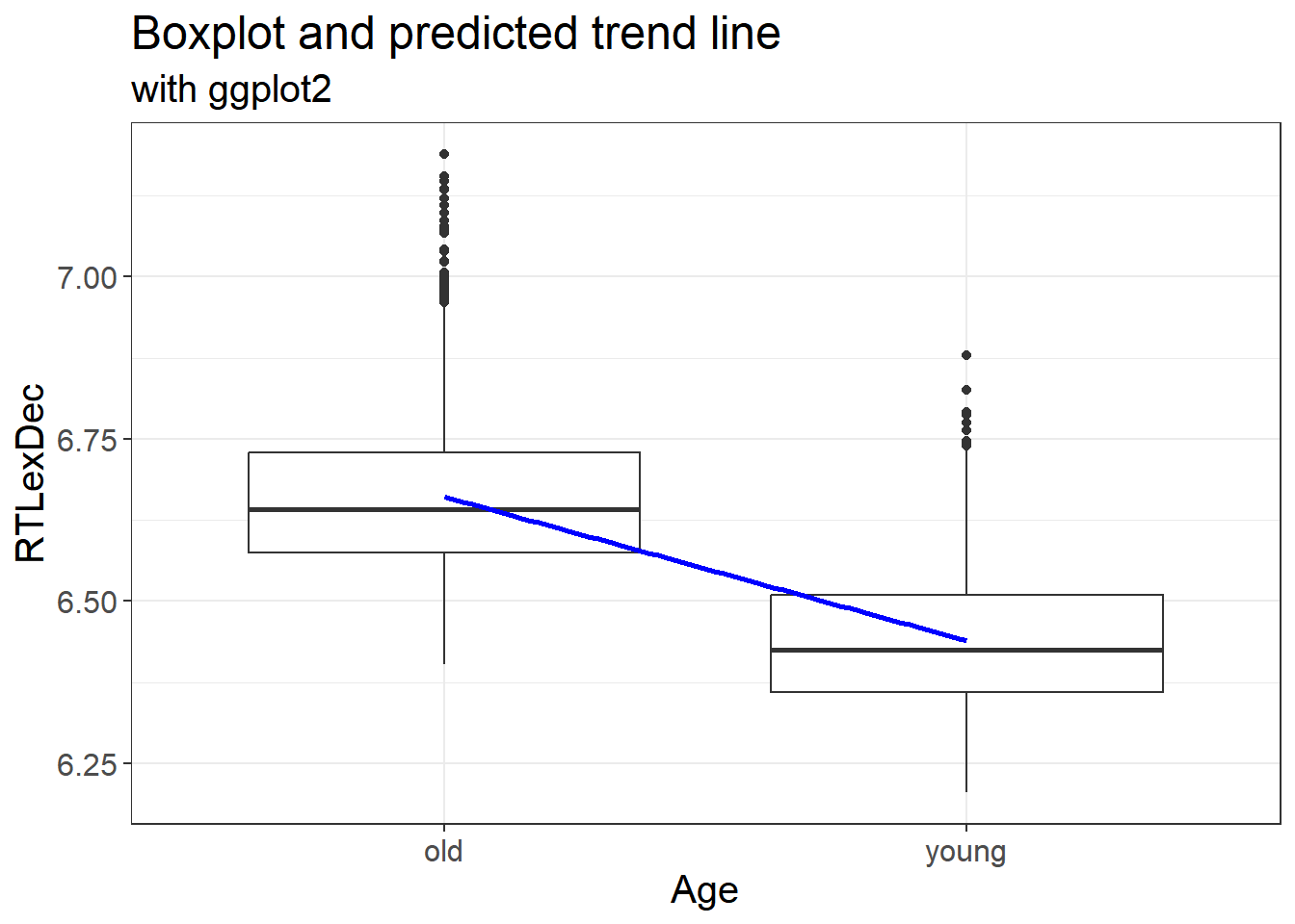

This allows us to plot the fitted values from our model with the predicted linear trend. This is exactly the same as our original data.

3.3.4.2 Predicted means and the trend line

We can also plot the predicted means and linear trend

english %>% 
  ggplot(aes(x = AgeSubject, y = predict(mdl.lm)))+
  geom_boxplot(color = "blue") +
  theme_bw() + theme(text = element_text(size = 15)) +
  geom_smooth(aes(x = as.numeric(AgeSubject), y = predict(mdl.lm)), method = "lm", color = "blue") + 
    labs(x = "Age", y = "RTLexDec", title = "Predicted means and trend line", subtitle = "with ggplot2")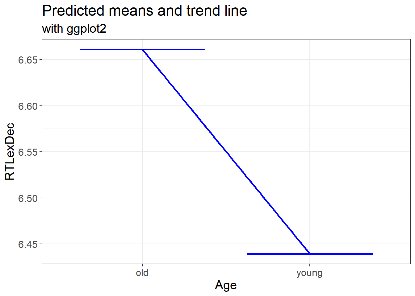

3.3.4.3 Raw data, predicted means and the trend line

We can also plot the actual data, the predicted means and linear trend

english %>% 
  ggplot(aes(x = AgeSubject, y = RTlexdec))+
  geom_boxplot() +
  geom_boxplot(aes(x = AgeSubject, y = predict(mdl.lm)), color = "blue") +
  theme_bw() + theme(text = element_text(size = 15)) +
  geom_smooth(aes(x = as.numeric(AgeSubject), y = predict(mdl.lm)), method = "lm", color = "blue") +
    labs(x = "Species", y = "Length", title = "Boxplot raw data, predicted means (in blue) and trend line", subtitle = "with ggplot2")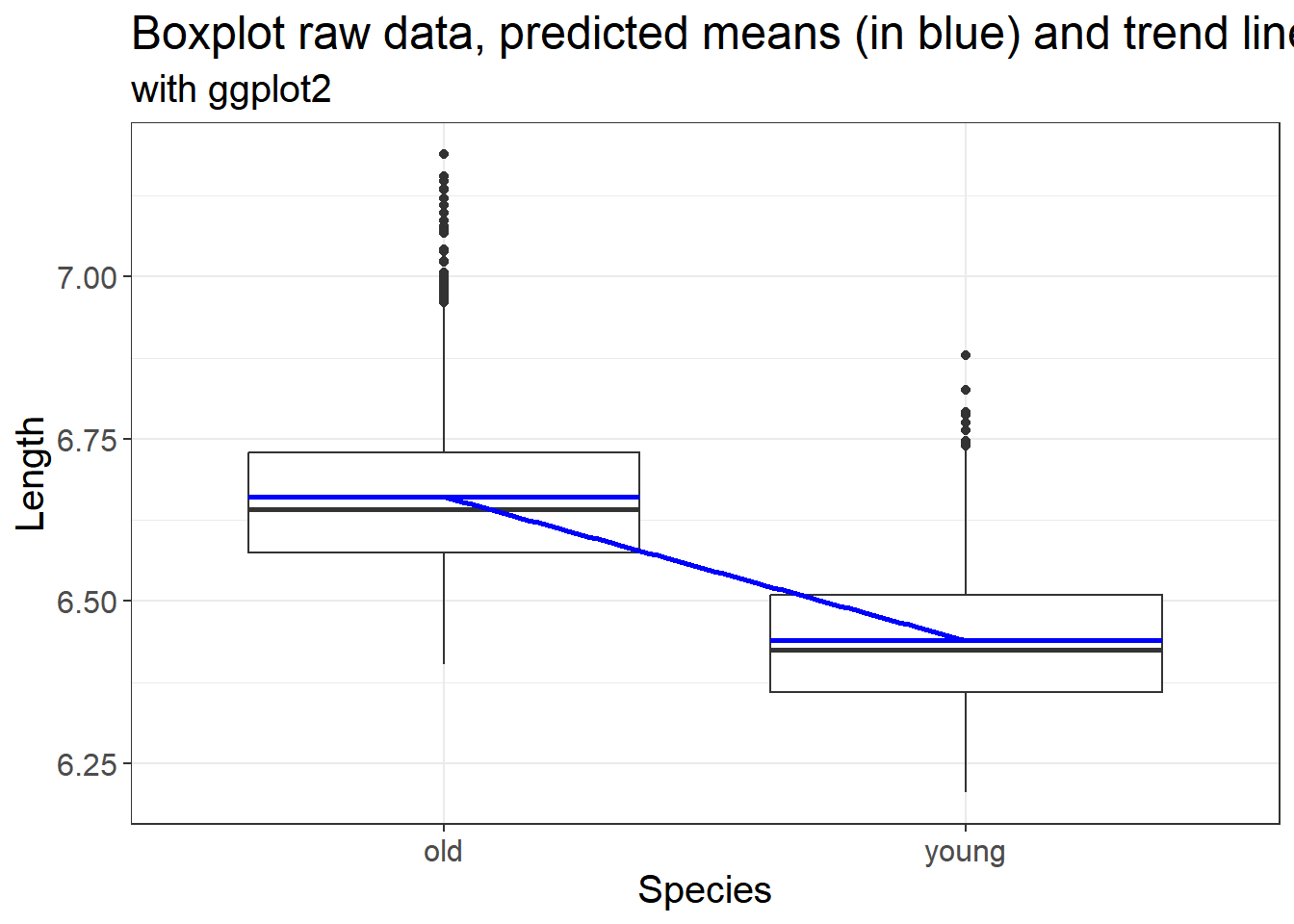

3.3.4.4 Add significance levels and trend line on a plot?

We can use the p values generated from either our linear model to add significance levels on a plot. We use the code from above and add the significance level. We also add a trend line

english %>% 
  ggplot(aes(x = AgeSubject, y = RTlexdec))+
  geom_boxplot() +
  geom_boxplot(aes(x = AgeSubject, y = predict(mdl.lm)), color = "blue") +
  theme_bw() + theme(text = element_text(size = 15)) +
  geom_smooth(aes(x = as.numeric(AgeSubject), y = predict(mdl.lm)), method = "lm", color = "blue") +
    labs(x = "Species", y = "Length", title = "Boxplot raw data, predicted means (in blue) and trend line", subtitle = "with significance testing") +
    geom_signif(comparison = list(c("old", "young")), 
              map_signif_level = TRUE, test = function(a, b) {
                list(p.value = summary(mdl.lm)$coefficients[2, 4])})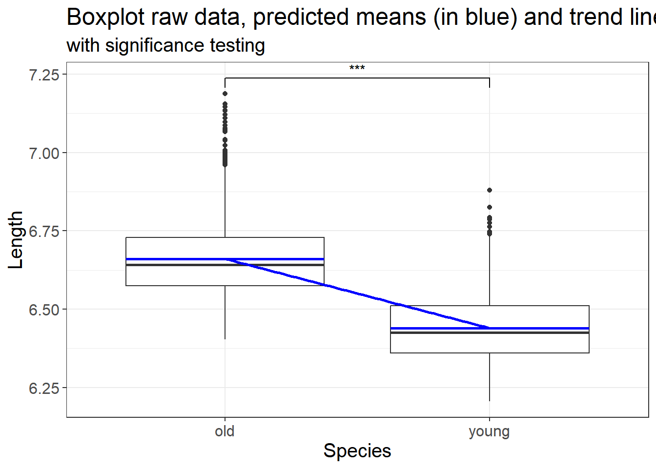

3.3.5 What about pairwise comparison?

When having three of more levels in our predictor, we can use pairwise comparisons, with corrections to evaluate differences between each level.

summary(mdl.lm)

## 
## Call:
## lm(formula = RTlexdec ~ AgeSubject, data = .)
## 
## Residuals:
##      Min       1Q   Median       3Q      Max 
## -0.25776 -0.08339 -0.01669  0.06921  0.52685 
## 
## Coefficients:
##               Estimate Std. Error t value Pr(>|t|)    
## (Intercept)   6.439237   0.002324 2771.03   <2e-16 ***
## AgeSubjectold 0.221721   0.003286   67.47   <2e-16 ***
## ---
## Signif. codes:  0 '***' 0.001 '**' 0.01 '*' 0.05 '.' 0.1 ' ' 1
## 
## Residual standard error: 0.1111 on 4566 degrees of freedom
## Multiple R-squared:  0.4992, Adjusted R-squared:  0.4991 
## F-statistic:  4552 on 1 and 4566 DF,  p-value: < 2.2e-16

mdl.lm %>% emmeans(pairwise ~ AgeSubject, adjust = "fdr") -> mdl.emmeans
mdl.emmeans

## $emmeans
##  AgeSubject emmean      SE   df lower.CL upper.CL
##  young       6.439 0.00232 4566    6.435    6.444
##  old         6.661 0.00232 4566    6.656    6.666
## 
## Confidence level used: 0.95 
## 
## $contrasts
##  contrast    estimate      SE   df t.ratio p.value
##  young - old   -0.222 0.00329 4566 -67.468  <.0001

How to interpret the output? Discuss with your neighbour and share with the group.

Hint… Look at the emmeans values for each level of our factor “Species” and the contrasts.

3.3.6 Multiple predictors?

Linear models require a numeric outcome, but the predictor can be either numeric or a factor. We can have more than one predictor. The only issue is that this complicates the interpretation of results

english %>% 
  lm(RTlexdec ~ AgeSubject * WordCategory, data = .) %>% 
  summary()

## 
## Call:
## lm(formula = RTlexdec ~ AgeSubject * WordCategory, data = .)
## 
## Residuals:
##      Min       1Q   Median       3Q      Max 
## -0.25079 -0.08273 -0.01516  0.06940  0.52285 
## 
## Coefficients:
##                                Estimate Std. Error  t value Pr(>|t|)    
## (Intercept)                    6.664955   0.002911 2289.950   <2e-16 ***
## AgeSubjectyoung               -0.220395   0.004116  -53.545   <2e-16 ***
## WordCategoryV                 -0.010972   0.004822   -2.275   0.0229 *  
## AgeSubjectyoung:WordCategoryV -0.003642   0.006820   -0.534   0.5934    
## ---
## Signif. codes:  0 '***' 0.001 '**' 0.01 '*' 0.05 '.' 0.1 ' ' 1
## 
## Residual standard error: 0.1109 on 4564 degrees of freedom
## Multiple R-squared:  0.5008, Adjusted R-squared:  0.5005 
## F-statistic:  1526 on 3 and 4564 DF,  p-value: < 2.2e-16

And with an Anova

english %>% 
  lm(RTlexdec ~ AgeSubject * WordCategory, data = .) %>% 
  anova()

## Analysis of Variance Table
## 
## Response: RTlexdec
##                           Df Sum Sq Mean Sq   F value    Pr(>F)    
## AgeSubject                 1 56.141  56.141 4564.2810 < 2.2e-16 ***
## WordCategory               1  0.173   0.173   14.0756 0.0001778 ***
## AgeSubject:WordCategory    1  0.004   0.004    0.2851 0.5933724    
## Residuals               4564 56.138   0.012                        
## ---
## Signif. codes:  0 '***' 0.001 '**' 0.01 '*' 0.05 '.' 0.1 ' ' 1

The results above tell us that all predictors used are significantly different.