10.6 Decision Trees
Decision trees are a statistical tool that uses the combination of predictors to identify patterns in the data and provides classification accuracy for the model.
The decision tree used is based on conditional inference trees that looks at each predictor and splits the data into multiple nodes (branches) through recursive partitioning in a tree-structured regression model. Each node is also split into leaves (difference between levels of outcome).
Decision trees via ctree does the following:
- Test global null hypothesis of independence between predictors and outcome.
- Select the predictor with the strongest association with the outcome measured based on a multiplicity adjusted p-values with Bonferroni correction
- Implement a binary split in the selected input variable.
- Recursively repeat steps 1), 2). and 3).
Let’s see this in an example using the same dataset. To understand what the decision tree is doing, we will dissect it, by creating one tree with one predictor and move to the next.
10.6.1 Individual trees
10.6.1.1 Tree 1
### from the package party
set.seed(42)
tree1 <- dfPharV2 %>%
  ctree(
    context ~ Z2mnZ1,
    data = .)
print(tree1)
##
## Conditional inference tree with 4 terminal nodes
##
## Response: context
## Input: Z2mnZ1
## Number of observations: 402
##
## 1) Z2mnZ1 <= 9.551456; criterion = 0.999, statistic = 11.678
## 2) Z2mnZ1 <= 6.779068; criterion = 1, statistic = 12.368
## 3) Z2mnZ1 <= 4.004879; criterion = 1, statistic = 56.773
## 4)* weights = 157
## 3) Z2mnZ1 > 4.004879
## 5)* weights = 106
## 2) Z2mnZ1 > 6.779068
## 6)* weights = 64
## 1) Z2mnZ1 > 9.551456
## 7)* weights = 75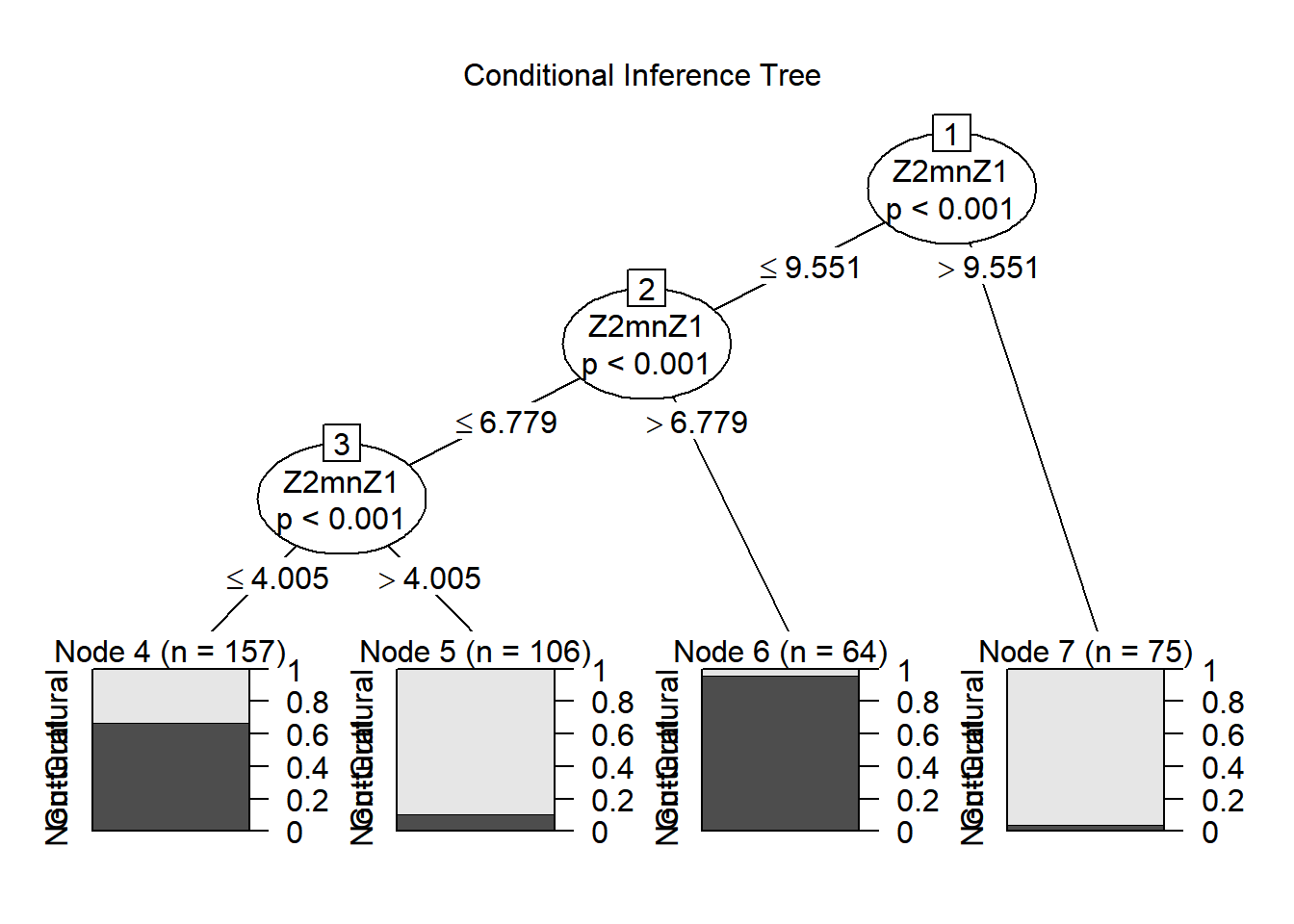
How to interpret this figure? Let’s look at mean values and a plot for this variable. This is the difference between F2 and F1 using the bark scale. Because gutturals are produced within the pharynx (regardless of where), the predictions is that a high F1 and a low F2 will be the acoustic correlates related to this constriction location. The closeness between these formants yields a lower Z2-Z1. Hence, the prediction is as follow: the smaller the difference, the more pharyngeal-like constriction these consonants have (all else being equal!). Let’s compute the mean/median and plot the difference between the two contexts.
dfPharV2 %>%
  group_by(context) %>%
  summarise(mean = mean(Z2mnZ1),
            median = median(Z2mnZ1),
            count = n())
## # A tibble: 2 × 4
## context mean median count
## <fct> <dbl> <dbl> <int>
## 1 Non-Guttural 6.30 5.02 222
## 2 Guttural 5.31 3.84 180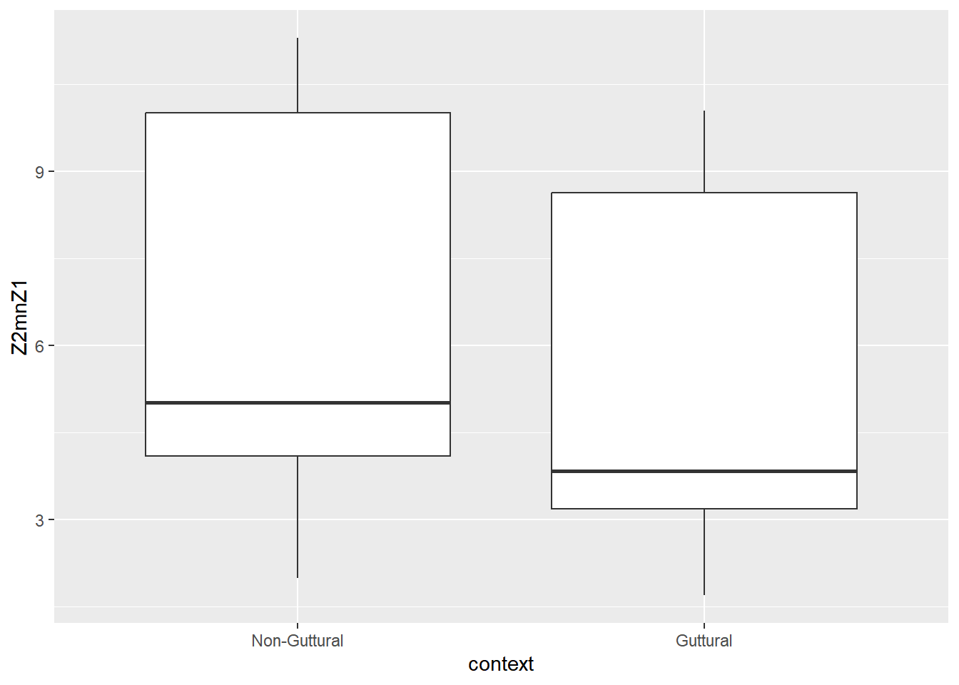
The table above reports the mean and median of Z2-Z1 for both levels of context and the plots show the difference between the two. We have a total of 180 cases in the guttural, and 222 in the non-guttural.
When considering the conditional inference tree output, various splits were obtained.
The first is any value higher than 9.55 being assigned to the non-guttural class (around 98% of 75 cases)
Then, with anything lower than 9.55, a second split was obtained. A threshold of 6.78: higher assigned to guttural (around 98% of 64 cases), lower, were split again with a threshold of 4 Bark. A third split was obtained: values lower of equal to 4 Bark are assigned to the guttural (around 70% of 157 cases) and values higher than 4 Barks assigned to the non-guttural (around 90% of 106 cases).
Dissecting the tree like this allows interpretation of the output. In this example, this is quite a complex case and ctree allowed to fine tune the different patterns seen with
Now let’s look at the full dataset to make sense of the combination of predictors to the difference.
10.6.2 Model 1
10.6.2.1 Model specification
##
##   Conditional inference tree with 8 terminal nodes
##
## Response:  context
## Inputs:  CPP, Energy, H1A1c, H1A2c, H1A3c, H1H2c, H2H4c, H2KH5Kc, H42Kc, HNR05, HNR15, HNR25, HNR35, SHR, soe, Z1mnZ0, Z2mnZ1, Z3mnZ2, Z4mnZ3, F0Bark, A1mnA2, A1mnA3, A2mnA3
## Number of observations:  402
##
## 1) A2mnA3 <= -13.78; criterion = 1, statistic = 42.329
##   2) Z4mnZ3 <= 1.592125; criterion = 1, statistic = 40.991
##     3) H2H4c <= -8.396333; criterion = 0.993, statistic = 13.141
##       4)*  weights = 8
##     3) H2H4c > -8.396333
##       5)*  weights = 100
##   2) Z4mnZ3 > 1.592125
##     6) Energy <= 2.8295; criterion = 0.999, statistic = 16.923
##       7)*  weights = 25
##     6) Energy > 2.8295
##       8)*  weights = 10
## 1) A2mnA3 > -13.78
##   9) H1H2c <= 10.27167; criterion = 0.953, statistic = 9.458
##     10) SHR <= 0.1566667; criterion = 1, statistic = 18.337
##       11)*  weights = 99
##     10) SHR > 0.1566667
##       12) H1H2c <= 0.7411667; criterion = 0.972, statistic = 10.449
##         13)*  weights = 103
##       12) H1H2c > 0.7411667
##         14)*  weights = 30
##   9) H1H2c > 10.27167
##     15)*  weights = 27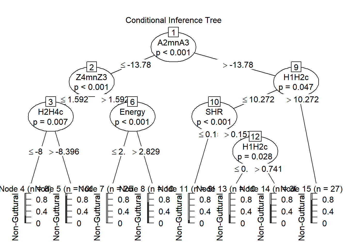
How to interpret this complex decision tree?
Let’s obtain the median value for each predictor grouped by context. Discuss some of the patterns.
## # A tibble: 2 × 24
##   context      CPP_mean Energy_mean H1A1c_mean H1A2c_mean H1A3c_mean H1H2c_mean
##   <fct>           <dbl>       <dbl>      <dbl>      <dbl>      <dbl>      <dbl>
## 1 Non-Guttural     26.4        5.28       16.5       12.5       4.62       3.85
## 2 Guttural         26.3        7.04       16.6       15.6       1.04       4.49
## # ℹ 17 more variables: H2H4c_mean <dbl>, H2KH5Kc_mean <dbl>, H42Kc_mean <dbl>,
## #   HNR05_mean <dbl>, HNR15_mean <dbl>, HNR25_mean <dbl>, HNR35_mean <dbl>,
## #   SHR_mean <dbl>, soe_mean <dbl>, Z1mnZ0_mean <dbl>, Z2mnZ1_mean <dbl>,
## #   Z3mnZ2_mean <dbl>, Z4mnZ3_mean <dbl>, F0Bark_mean <dbl>, A1mnA2_mean <dbl>,
## #   A1mnA3_mean <dbl>, A2mnA3_mean <dbl>
We started with context as our outcome, and all 23 acoustic measures as predictors. A total of 8 terminal nodes were identified with multiple binary splits in their leaves, allowing separation of the two categories. Looking specifically at the output, we observe a few things.
The first node was based on A2*-A3*, detecting a difference between non-gutturals and gutturals. For the first binary split, a threshold of -13.78 Bark was used (mean non guttural = -7.86; mean guttural = -14.58), then for values lower of equal to this threshold, a second split was performed using Z4-Z3 (mean non guttural = 1.67; mean guttural = 1.43) with any value smaller and equal to 1.59, then another binary split using H2*-H4*, etc…
Once done, the ctree provides multiple binary splits into guttural or non-guttural.
Any possible issues/interesting patterns you can identify? Look at the interactions between predictors.
10.6.2.2 Predictions from the full model
Let’s obtain some predictions from the model and evaluate how successful it is in dealing with the data.
##
## pred.ctree     Non-Guttural Guttural
##   Non-Guttural          194       41
## Guttural 28 139## PCC PCC.sd
## 1 0.8283582 0.01882992## specificity specificity.sd
## 1 0.7722222 0.03134731## sensitivity sensitivity.sd
## 1 0.8738739 0.02233216## Setting levels: control = Non-Guttural, case = Guttural## Setting direction: controls < cases##
## Call:
## roc.default(response = dfPharV2$context, predictor = as.numeric(pred.ctree))
##
## Data: as.numeric(pred.ctree) in 222 controls (dfPharV2$context Non-Guttural) < 180 cases (dfPharV2$context Guttural).
## Area under the curve: 0.823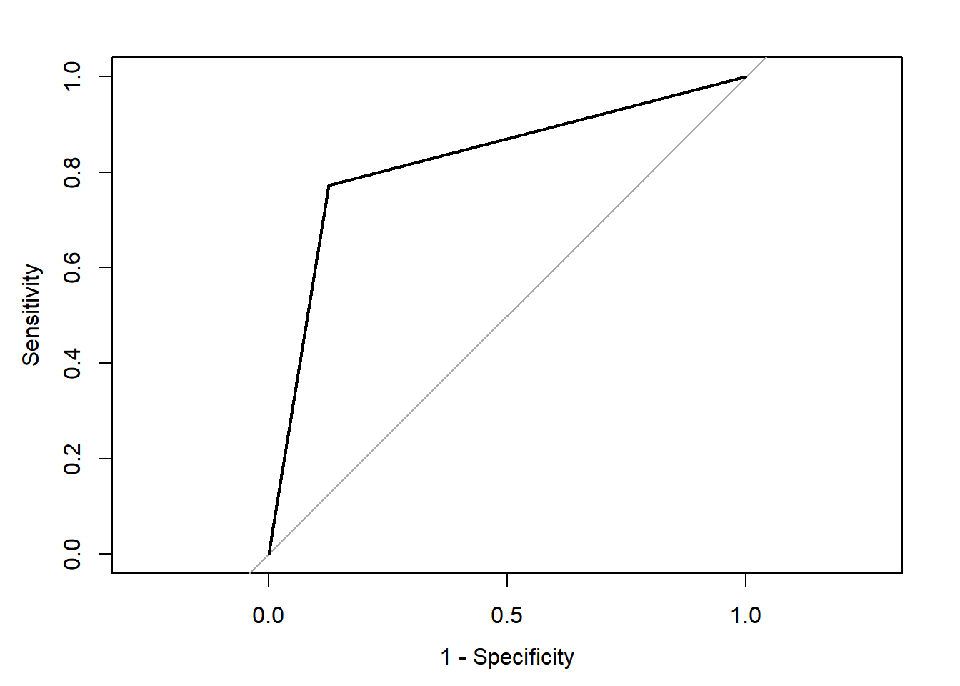
This full model has a classification accuracy of 82.8%. This is not bad!! It has a relatively moderate specificity at 0.772 (at detecting the gutturals) but a high sensitivity at 0.874 (at detecting the non-gutturals). The ROC curve shows the relationship between the two with an AUC of 0.823. This is a good model, but it is not perfect. The confusion matrix shows that the model was able to detect 80% of the gutturals, but 20% were misclassified as non-gutturals. The opposite is true for the non-gutturals: 80% were detected, but 20% were misclassified as gutturals. The AUC is at 0.823, which is not too bad. ### Random selection
One important issue is that the trees we grew above are biased. They are based on the full dataset, which means they are very likely to overfit the data. We did not add any random selection and we only grew one tree each time. If you think about it, is it possible that we obtained such results simply by chance?
What if we add some randomness in the process of creating a conditional inference tree?
We change a small option in ctree to allow for random selection of variables, to mimic what Random Forests will do. We use controls to specify mtry = 5, which is the rounded square root of number of predictors.
10.6.2.3 Model 2
set.seed(42)
fit1 <- dfPharV2  %>%
  ctree(
    context ~ .,
    data = .,
    controls = ctree_control(mtry = 5))

plot(fit1, main = "Conditional Inference Tree")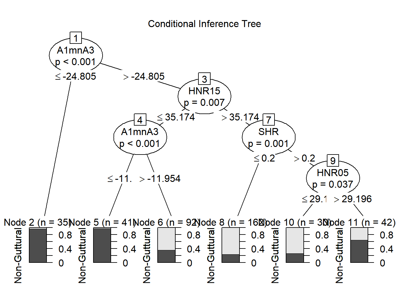
##
## pred.ctree1    Non-Guttural Guttural
##   Non-Guttural          205       79
## Guttural 17 101## PCC PCC.sd
## 1 0.761194 0.0212911## specificity specificity.sd
## 1 0.5611111 0.03709157## sensitivity sensitivity.sd
## 1 0.9234234 0.01788761## Setting levels: control = Non-Guttural, case = Guttural## Setting direction: controls < cases##
## Call:
## roc.default(response = dfPharV2$context, predictor = as.numeric(pred.ctree1))
##
## Data: as.numeric(pred.ctree1) in 222 controls (dfPharV2$context Non-Guttural) < 180 cases (dfPharV2$context Guttural).
## Area under the curve: 0.7423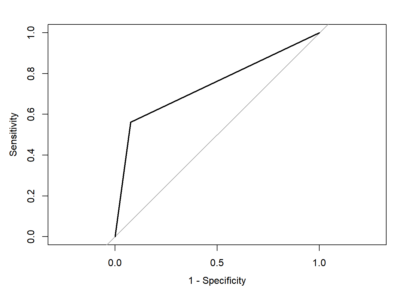
Can you compare results between you and discuss what is going on?
When adding one random selection process to our ctree, we allow it to obtain more robust predictions. We could even go further and grow multiple small trees with a portion of datapoints (e.g., 100 rows, 200 rows). When doing these multiple random selections, you are growing multiple trees that are decorrelated from each other. These become independent trees and one can combine the results of these trees to come with clear predictions.
This is how Random Forests work. You would start from a dataset, then grow multiple trees, vary number of observations used (nrow), and number of predictors used (mtry), adjust branches, and depth of nodes and at the end, combine the results in a forest. You can also run permutation tests to evaluate contributions of each predictor to the outcome. This is the beauty of Random Forests. They do all of these steps automatically at once for you!