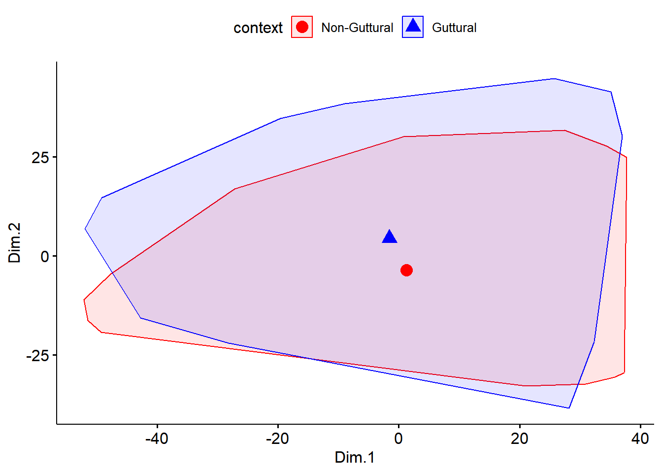
9.6 Multidimensional scaling

In this section, we explore multidimensional scaling. This is another unsupervised learning algorithm. As with cluster analysis, we start by running the MDS algorithm and use Kmeans clustering to allow visualisation of the two-dimensional data. Usually, up to 5 dimensions explain a large percentage of the variance in the data; in our case, we only go for 2 dimensions to evaluate how the two groups are close (or not) to each other). As with cluster analysis, we could compute number of clusters; something we are not doing here.

9.6.1 Computing MDS

We perform a MDS Clustering with 2 Clusters. We use a Euclidean distance matrix. See here for details on the available dissimilarity methods.

dat1MDS <- dfPharPCA

set.seed(123)

mds.resdat1 <- dat1MDS[-1] %>%
  dist(method = 'euclidean') %>%          
  cmdscale() %>%
  as_tibble()
colnames(mds.resdat1) <- c("Dim.1", "Dim.2")

mds.resdat1 %>% head(10)

## # A tibble: 10 × 2
##    Dim.1 Dim.2
##    <dbl> <dbl>
##  1 -45.4 10.1 
##  2 -24.6  1.90
##  3 -52.0  6.85
##  4 -36.1 19.9 
##  5 -25.2 11.3 
##  6 -40.5 10.1 
##  7 -40.8 12.0 
##  8 -38.0  3.41
##  9 -30.2 10.3 
## 10 -19.5  5.61

9.6.2 Kmeans clustering

## K-means clustering
clust <- kmeans(mds.resdat1, 2)$cluster %>%
  as.factor()
mds.resdat1 <- mds.resdat1 %>%
  mutate(groups = clust)
mds.resdat1$context <- dat1MDS$context

9.6.3 Plot

## Plot and color by groups
ggscatter(mds.resdat1, x = "Dim.1", y = "Dim.2", col = "context",
          label = NULL,
          color = "context",
          palette = c("red", "blue"),
          size = 2, 
          ellipse = TRUE,
          ellipse.type = "convex",
          repel = FALSE,
          shape = "context",
          point = FALSE,
          mean.point = TRUE)